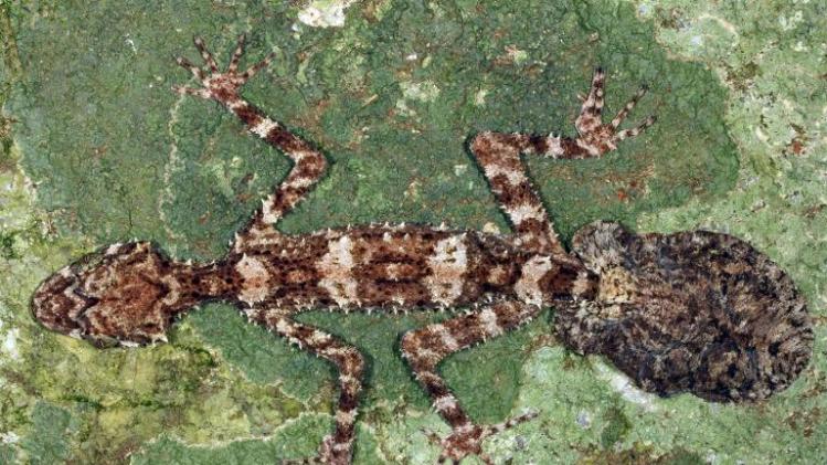
In 1975, vertebrate paleontologist L.B. Halstead pointed out that the rhomboidal flippers seen in the Rines Loch Ness underwater photos from 1972 did not match the hydrofoil shape of then-current reconstructions of plesiosaur flipper shapes, based on skin outlines preserved around some plesiosaur flipper specimens (Hydrodrion brachypterygius and Seelyosaurus guillelmi-imperatoris). A May 2013 Mast
...er’s thesis by vertebrate paleontologist Mark Cruz DeBlois may question that assertion. Using hydrodynamic principles in combination with advanced mathematical formulas, DeBlois has produced a predicted plesiosaur flipper shape for the front flippers of the plesiosaur Cryptocleidus eurymerus that is much closer to the rhomboidal shape of the Rines flippers, with a much larger trailing edge of flesh that extends beyond the flipper bones (see upper left, blue and red outlines). Read it for yourself athttp://mds.marshall.edu/cgi/viewcontent.cgi?article=1502&context=etd

DeBlois' hypothesized front flipper of Hydrodrion brachypterygius overlayed on the second
Rines "flipper"photo image
Traditional reconstructions of plesiosaur flipper morphology and plesiosaur flipper skin impressions: (clockwise from top left) the front and rear flippers of Hydrodrion brachypterygius, the right rear flipper of the "Collard plesiosaur" from the UK, a typical model of the traditional proposed plesiosaur flipper morphology and sketches of the skin impressions surrounding the flippers of the plesiosaurs Seelyosaurus guillelmi-imperatoris and Hydrodrion brachypterygius.
Below is the full text of the source. I have left off the Appendix. Unfortunately Blogger is not being very helpful again and so this time I figured just including the text would be enough (Instead of trying to restore it to the original appearance, which is what I usually do.)
Marshall University
Marshall Digital Scholar
Theses, Dissertations and Capstones
1-1-2013
Quantitative Reconstruction and Two-
Dimensional, Steady Flow Hydrodynamics of the
Plesiosaur Flipper
Mark Cruz DeBlois
deblois@marshall.edu
Follow this and additional works at:
http://mds.marshall.edu/etd
Part of the Aquaculture and Fisheries Commons, and the Terrestrial and Aquatic Ecology
Commons
This Thesis is brought to you for free and open access by Marshall Digital Scholar. It has been accepted for inclusion in Theses, Dissertations and
Capstones by an authorized administrator of Marshall Digital Scholar. For more information, please contact zhangj@marshall.edu.
Recommended Citation
DeBlois, Mark Cruz, "Quantitative Reconstruction and Two-Dimensional, Steady Flow Hydrodynamics of the Plesiosaur Flipper"
(2013). Theses, Dissertations and Capstones. Paper 501.
QUANTITATIVE RECONSTRUCTION AND TWO-DIMENSIONAL, STEADY
FLOW HYDRODYNAMICS OF THE PLESIOSAUR FLIPPER
Thesis submitted to
the Graduate College of
Marshall University
In partial fulfillment of
the requirements for the degree of
Master of Science
in Biological Science
By
Mark Cruz DeBlois
Approved by
Dr. F. Robin O’Keefe, Ph.D., Advisor, Committee Chairperson
Dr. Paul Constantino, Ph.D.
Dr. Suzanne Strait, Ph.D.
Marshall University
May 2013
DeBlois
ii
ii
ACKNOWLEDGEMENTS
I would like to thank Robin O’Keefe for his tireless mentorship inside the lab and his
friendship outside. He has guided me through the threshold of not just the field of paleontology
but also functional morphology and biomechanics. Second I would like to thank James Denvir
from Marshall University. The parsing script that Jim wrote for this project made it possible to
handle and analyze enormous amounts of data. Without his code, this project would not have
attained the scope that it has now. I would also like to thank Mark Menor, my dear friend from
the University of Hawaii, Manoa. Mark has been my guide as I learned to write code in general
and in Matlab specifically. I would have been utterly lost in the world of computer programming
without his help. I would like to thank my comrades in arms at Robin’s paleo lab: Josh Corrie,
Christina Byrd, and Alex Brannick. They have been there to cheer and commiserate with me
through the ups and downs of this project. I would like to thank Lyndsay Rankin. She has been
my biggest fan and tireless supporter. Lastly I would like to thank my family who has and will
always be there behind me to provide support, encouragement, and solace. You all have made
this project possible. To all of you, thank you.
DeBlois
iii
iii
This project is dedicated to my family especially Papa and Mama.
I love you all.
DeBlois
iv
iv
TABLE OF CONTENTS
List of Tables.……………………………………………………………………………………..v
List of Figures……………….……………………………………………………………………iv
List of Variables…….…….………………………………………………………………………ix
List of Equations………….…………………………………………………………………...…xii
Abstract……………………………………………………………………………………………1
Introduction………………………………………………………………………………………..2
Chapter 1: Background…………………………………………………………………………...3
Plesiosauria………………………………………………………………………………..3
Distribution and Phylogeny……………………………………………………….3
Morphotypes………………………………………………………………………8
Properties of Hydrofoils………………………………………………………………….10
Sources of Lift and Drag…………………………………………………………10
Flow Effects on Lift and Drag…………………………………………………...13
Shape Effects on Lift and Drat…………………………………………………..15
Study Parameters…………………………………………………………......….17
Biological Hydrofoils………………………………………………………………........18
Extant Hydrofoil-Bearing Tetrapods…………………………………………….18
Anatomical Composition………………………………………………………...19
Trends in Shape……………………………………………………………….....20
Plesiosaur Hydrofoil and Locomotion…………………………………………………...21
Summary and Rationale………………………………………………………………….25
DeBlois
v
v
Chapter 2: Shape and Hydrodynamics of the plesiosaur flipper………………………………...26
Introduction………………………………………………………………………………26
Method………………………………………………………………………………...…29
Inferring Shape from Fossil Specimens………………………………………….29
Specimen…………………………………………………………………30
Image Pre-Processing……………………………………………………30
Estimating the Leading Edge………………………………………….…31
Estimating the Trailing Edge…………………………………………….31
Results……………………………………………………………………………………43
Cryptoclidus eurymerus Femur Hydrofoil ………………………………………43
Cryptoclidus eurymerus Humerus Hydrofoil…………………………………….44
Discussion……………………………………………………………………………..…52
Chapter 3: Future Work – Validation Experiments……………………………………………..59
Introduction………………………………………………………………………………59
Method……………………………………………………………………………...……59
Preliminary Data…………………………………………………………………………59
Interpretation……………………………………………………………………………..60
Chapter 4: Future Work – Plesiosaur Flipper Kinematic Hypothesis…………………………...61
DeBlois
vi
vi
Introduction………………………………………………………………………………61
Method…………………………………………………………………………………...61
Preliminary Data………………..………………………………………………………..62
Interpretation……………………………………………………………………………..63
Chapter 5: Future Work – Functional Evolution of the Shape of Plesiosaur Flippers………….66
Introduction………………………………………………………………………………66
Methods…………………………………………………………………………………..66
Preliminary Data…………………………………………………………………………67
Interpretation……………………………………………………………………………..67
Chapter 6: Future Work – Three-Dimensional Models…………………………………………69
Literature Cited…………………………………………………………………………………..70
Appendix…………………………………………………………………………………………77
Custom Matlab Script……………………..……………………………………………………..77
IRB Letter………………………………………………………………………………………..90
DeBlois
vii
vii
LIST OF TABLES
Table 1: Defining characteristics of plesiosauromorph and pliosauromorph body plans………...9
Table 2: Geometry and hydrodynamics of the reconstructed plesiosaur hydrofoils…………....51
Table 3: Inviscid hydrodynamics of the cetacean, plesiosaur, and engineered hydrofoils……...51
DeBlois
viii
viii
LIST OF FIGURES
Figure 1: Plesiosaur body plans…………...…………...…………...………….............................5
Figure 2: Phylogenetic tree of Sauropterygia…………...…………...…………...…………........6
Figure 3: Phylogenetic tree of Plesiosauria…………...…………...…………...…………...........7
Figure 4: Diagram of hydrofoil cross-section and hydrodynamic forces……………………….11
Figure 5: Plesiosaur flipper planform shape…………...…………...…………...…………........23
Figure 6: Biological hydrofoils…………...…………...…………...…………............................28
Figure 7: Skeletal reconstruction of the Cryptoclidus eurymerus…………...………...……......40
Figure 8: Flowchart of the trailing edge reconstruction…………...…………...…………...…...41
Figure 9: Sample contour plot…..…………...…………...…………...…………........................42
Figure 10: Contour plots for C. eurymerus femur…………...…………...…………...…………45
Figure 11: The best functional hydrofoil shape for the C. eurymerus femur…………...……….46
Figure 12: Contour plots for C. eurymerus humerus……….…………...………….....…………47
Figure 13: The best functional hydrofoil shape for the C. eurymerus humerus………...……….48
Figure 14: The humerus and femur hydrofoils and similarly shaped engineered hydrofoils……50
Figure 15: Planform reconstruction for the C. eurymerus fore and hind flippers………………..55
Figure 16: The effect of Reynolds number (Re) on the contour plot topography………..……...60
Figure 17: Possible changes in hydrofoil shape during the stroke cycle……….…………...…...63
Figure 18: Reconstructed hydrofoil shapes for varios taxa within Plesiosauria……….…… 67-68
DeBlois
ix
ix
LIST OF VARIABLES
Re = Reynolds number
U = velocity of flow
η = kinematic viscosity of water (η = 1.0x10⁻⁶ m2/s)
CL = coefficient of lift
CD = coefficient of drag
CP = coefficient of pressure
Cf = skin-friction coefficient
Cdissipation - the dissipation coefficient
S = hydrofoil surface area
ρ = density of fluid
L = lift
D = drag
!
C(") == c"las•s (f1u#nc"ti)o1n
x = x-coordinate
c = chord length
!
" =
x
c
!
S(") n!
r!(n # r)! r=0
n$
•"r • (1#")=
shape function n #r
n = order of the Bernstein Polynomial (n = 3)
S(") =
n!
r!(n # r)! r=0
n$
•"r • (1#")= binomial cno#refficient
DeBlois
x
x
Ar = CST coefficient to be set using leas-squares fitting (A1 to A4)
!
Z(") = function of the parameterized hydrofoil
!
zTE,top = trailing edge tip y-value for the top half (= 0)
!
"ztop =
zTE,top
c
= thickness of the trailing edge tip of the top half (= 0)
!
zTE,bottom = trailinge edge tip y-value for the bottom half (= 0)
!
"zbottom =
zTE,bottom
c
= thickness of the trailing edge tip of the bottom half (= 0)
Φ = the streamfunction
γ = vortex distribution
σ = strength of the source distribution
x,y = x,y-coordinates of a point on the flow field
s = a point along the panel
r = magnitude of the vector between the points x,y and s
α = angle of the vector between the points x,y and s
!
q" = freestream velocity
!
u" =
!
q" cos# , component of
!
q"
!
v" =
!
q" sin# , component of
!
q"
!
x = x cos" + y sin"
uedge = flow velocity at the edge of the boundary layer
H = shape parameter
H* = kinetic energy shape parameter
H** = the density shape parameter
θ = boundary layer thickness
DeBlois
xi
xi
ξ = boundary layer coordinate
M = Mach number
Medge = Mach number at the edge of the boundary layer (Medge = 0)
Reθ = Reynolds number multiplied by θ
!
n˜ = amplitude of the largest Tollmien-Schlichting wave
ω = aerodynamic frequency parameter (also known as the reduced frequency value)
f = wingbeat frequency
DeBlois
xii
xii
LIST OF EQUATIONS
Equation 1: Re = cU/η …………...………...…………...…………........................................14
Equation 2a: L = 1/2ρSU2CL …………...………...…………...…………................................14
Equation 2b: D = 1/2ρSU2CD…………...………...…………...…………................................14
Equation 3:
!
C(") = " (1#")1…………...………...…………...………….............................32
Equation 4:
!
S(") =
n!
r!(n # r)! r=0
n$
Ar"r (1#")n #r
!
C(") = " (1#")1…………...……….........…32
Equation 5:
!
Z(") = " (1#")
n!
r!(n # r)! r=0
n$
Ar"r (1#")n #r…...……………………..….........…32
Equation 6:
!
Z(")top = " (1#") A1(1#")3 + A2(1#")2" + A3(1#") "2 + A4"3 ( ) +"$ztop ......…..33
Equation 7:
!
Z(")bottom = " (1#") A1(1#")3 + A2 (1#")2" + A3 (1#") "2 + A4"3 ( ) +"$zbottom…………33
Equation 8:
!
"(x, y) = u#y $ v#x +
1
2%
' & (s) lnr(s;x, y)ds + 1
2%
'( (s))(s;x, y)ds………….…35
Equation 9:
!
"(x, y) =
1
2#
% $ (s) lnr(s;x, y)ds + 1
2#
%& (s)'(s;x, y)ds……………………….…36
Equation 10:
!
Cp " #2
$ %
$x
q&
…...……………………..….....................................................…36
Equation 11:
!
CL = Cp " dx ...……………………..……........................................................…36
Equation 12:
!
CD = 2" (uedge /q#)(H +5) / 2…………………..……..............................................…36
Equation 13:
!
d"
d#
+ 2 + H $ Medge ( ) "
uedge
duedge
d#
=
Cf
2
…………..……...................................…37
Equation 14:
!
"
dH*
d#
+ 2H** + H*( (1$ H)) "
uedge
duedge
d#
= 2Cdissipation $ H* Cf
2
..........................…37
DeBlois
xiii
xiii
Equation 15: H* = H*(Hk, Medge, Reθ ) …….........................................................................…38
Equation 16: H** = H**(Hk, Medge ) …….............................................................................…38
Equation 17: Cf = Cf (Hk, Medge, Reθ ) ……...........................................................................…38
Equation 18: CD = CD (Hk, Medge, Reθ ) ……............................................................................38
Equation 19:
!
dn˜
d"
=
dn˜
dRe#
(Hk )
dRe#
d"
(Hk ,# )…….....................................................................38
Equation 20: ω = 2πƒc/U.........................................................................................................56
DeBlois
1
1
ABSTRACT
Plesiosaurs are a group of extinct marine reptiles that thrived during the Mesozoic Era.
They are unique for swimming with two hydrofoil-shaped flippers. Penguins, sea turtles, and
cetaceans all have hydrofoil shaped flippers but penguins and sea turtles only use the front pair to
produce thrust and cetaceans use their tail flukes. Consequently, the mode of swimming for
plesiosaurs has long been debated. However, a quantitative study of the hydrodynamic
properties of the flippers, which would constrain inference about their mode of swimming, has
not yet been done. The main reason is that the trailing edge of the plesiosaur flipper is made up
of soft tissue and does not fossilize. I present in this study a way to quantitatively reconstruct the
shape of the functional flipper hydrofoil of the plesiosaurs. Subsequently, I present the first
quantitative description of the hydrodynamic properties of plesiosaur flippers.
DeBlois
2
2
INTRODUCTION
Plesiosaurs are a group of extinct secondarily marine tetrapods unique for evolving two
pairs of hydrofoil-shaped flippers (Figure 1) (Robinson, 1975, 1977; Massare, 1994; Carpenter et
al., 2010). Other animals, like penguins and sea turtles, also have hydrofoil-shaped flippers but
these animals have distinctly different forelimb and hind limb morphologies, and rely primarily
on the forelimbs for swimming (Massare, 1994; Dodd, 1988; Wyneken, 1997; Davenport et al.,
1984). Since there are no extant modern analogs to plesiosaurs, their manner of locomotion has
long been debated. Prior studies on plesiosaur flipper anatomy suggest that they likely propelled
the animal by producing lift (De La Beche and Conybeare, 1821; Robinson, 1975; Brown, 1981;
Taylor, 1981; Frey and Reiss, 1982; Tarsitano and Reiss, 1982; Massare, 1994; Carpenter et al.,
2010), raising the possibility that plesiosaurs ‘flew’ through the water. However, others assert
that the flippers propelled the animal by pushing against the fluid acting as rowing paddles
instead of hydrofoils (Watson, 1924). Some have proposed a combination of the two with the
forelimbs producing lift while the hind limbs push against the water (Tarlo, 1957). Still others
have proposed a swimming motion similar to otariids (sea lions) (Godfrey, 1984). Despite the
keen interest in plesiosaur locomotion, no one has yet directly studied the hydrodynamics of
plesiosaur flippers. The widely held contemporary view (Storrs, 1993; O’Keefe, 2001b;
Carpenter et al., 2010) is that plesiosaur flippers produced lift, but because no one has yet
quantified the hydrodynamic properties of the flippers, the amount of lift (and drag) produced by
the flipper is unknown. The present study is the first to quantitatively investigate the
hydrodynamics of plesiosaur flippers from a variety of different plesiosaur taxa. Moreover since
locomotion plays a vital role in an animal’s biology, understanding the hydrodynamics of the
flippers will provide insight into and constrain inference about plesiosaur biology.
DeBlois
3
3
CHAPTER 1: BACKGROUND
PLESIOSAURIA
Distribution and Phylogeny
The Infra-order Plesiosauria, de Blainville 1835 (literally “near-lizards”) comprises a
monophyletic clade of extinct fully aquatic Mesozoic marine reptiles (O’Keefe, 2001a; Ketchum
and Benson, 2010). They first appeared in the Rhaetian during the late Triassic Period
approximately 200 million years ago (Mya) (Storrs, 1993, 1997; Rieppel, 1997) and thrived until
the mass extinction event at the Cretaceous – Tertiary (K-T) boundary approximately 65 Mya
(Storrs, 1997). During their 135 million year reign, plesiosaurs established a worldwide
distribution extending from North America (Nicholls and Russell, 1990) to Europe (Andrews,
1913), north to Greenland (von Huene, 1935 cited in Smith, 2007) and south to Australia and
New Zealand (Kear, 2003; Kear et al., 2006; Cruickshank and Fordyce, 2003). Plesiosaurs are
the most derived and successful members of the Order Sauropterygia, Owen 1860 (see Figure 2;
Rieppel, 2000; O’Keefe, 2001a; Storrs, 1997; Druckenmiller and Russell, 2008; Ketchum and
Benson, 2010). Plesiosauria is most closely related to Pistosauridae and other plesiosaur-like
nothosaurs (nothosaur-grade taxa), altogether comprising the subclade Pistosauroidea (Rieppel,
2000; O’Keefe, 2001a; Druckenmiller and Russell, 2008). In turn, Pistosauroidea together with
the subclades Nothosauria and Pachypleurosauroidea comprise the clade Eosauropterygia.
Finally, Eosauropterygia and Placodontia comprise Sauropterygia (see Figure 2; Rieppel, 2000;
O’Keefe, 2001a; Druckenmiller and Russell, 2008). Sauropterygia originated in the Upper
Permian and likely descended from primitive terrestrial diapsid reptiles (Carroll, 1981; Storrs,
1993; Neenan et al., 2013).
DeBlois
4
4
Plesiosauria is divided into two monophyletic superfamilies: Plesiosauroidea and
Pliosauroidea (O’Keefe, 2001a; Ketchum and Benson, 2010; Benson et al., 2012).
Plesiosauroidea consists of five families: Plesiosauridae, Elasmosauridae, Cryptoclididae,
Leptocleididae, and Polycotylidae (see Figure 3; Ketchum and Benson, 2010). Pliosauroidea
consists of two major families: Rhomaleosauridae and Pliosauridae (see Figure 3; O’Keefe,
2001a; Ketchum and Benson, 2010; Benson et al., 2012). Plesiosauridea are basal plesiosauroids
whereas Elasmosauridae, and Polycotylidae are derived crown group plesiosauroids. Likewise,
Rhomaleosauridae are basal pliosauroids whereas Pliosauridae are derived crown group
pliosauroids (O’Keefe 2001a; Ketchum and Benson, 2010; Benson et al., 2012). However,
recent work by Benson and colleagues (2012) suggest that Pliosauroidea constitutes a
paraphyletic group. In this scheme, Pliosauridae forms a monophyletic clade with
Plesiosauroidea (Neoplesiosauria) with Rhomaleosauridae as the immediate outgroup (Benson et
al., 2012). The phylogenetic position of Polycotylidae has fluctuated between the two
superfamilies owing to its similarity to both (Figure 1) with some authors placing it within
Pliosauroidea (Andrews, 1910, 1913; Welles, 1952; Brown, 1981; Brown and Cruickshank,
1994) while others authors place it in Plesiosauroidea (O’Keefe, 2001a, 2002; Ketchum and
Benson, 2010 and references therein). However since the most recent phylogenetic analysis of
Plesiosauria by Ketchum and Benson (2010) places Polycotylidae firmly in Plesiosauroidea,
Polycotylidae will be treated as belonging to Plesiosauroidea for the present study.
DeBlois
5
5
Figure 1. Representative plesiosauromorph and pliosauromorphs. Not to scale. (A)
Hydrotherosaurus, a plesiosauromorph belonging to Elasmosauridae in the superfamily
Plesiosauroidea. Lateral view. From O’Keefe, 2002. (B) Polycotylus, a pliosauromorph
belonging to Polycotylidae in the superfamily Plesiosauroidea. Top view. Adapted from
O’Keefe, 2009. (C) Liopleurodon, a pliosauromorph belonging to Pliosauridae in the
superfamily Pliosauroidea. Lateral view. From O’Keefe, 2002.
A
B
C
DeBlois
6
6
Figure 2. Cladogram showing the interrelationships within the Order Sauropterygia based on
work by Rieppel (2000).
DeBlois
7
7
Figure 3. Phylogenetic tree from Ketchum and Benson (2010) showing the relationships of taxa
within Plesiosauria as well as their respective temporal distributions. Note the positions of
Elasmosauridae and Polycotylidae within Plesiosauroidea and Pliosauridae within Pliosauroidea.
DeBlois
8
8
Morphotypes
Plesiosauria has traditionally been divided into two groups based on body plans
(morphotypes) (for a list of defining characters see Table 1) (Brown, 1981; O’Keefe, 2001b,
2002; Ketchum and Benson, 2010). Those with relatively small heads and long necks (labeled as
plesiosauromorphs) were traditionally grouped together and considered taxonomically distinct
from those with relatively large heads and short necks (labeled as pliosauromorphs, see Figure 1)
(Andrews, 1910, 1913; Welles, 1952; Brown, 1981; Brown and Cruickshank, 1994). This
dichotomy was challenged as early as 1907 by Williston and recent work has shown that the
pliosauromorph body plan likely evolved independently in several different lineages (Carpenter,
1997; O’Keefe, 2001a, 2002; Ketchum and Benson, 2010; Benson et al., 2012). The
plesiosauromorph – pliosauromorph dichotomy, therefore, does not correspond to any
phylogenetic division within Plesiosauria and, instead, represents a polyphyletic assemblage of
taxa. Pliosauridae, Rhomaleosauridae, and Polycotylidae all have the pliosauromorph body
plans but Polycotylidae is more closely related to Elasmosauridae, a plesiosauromorph, than to
either Pliosauridae or Rhomaleosauridae (see Figure 3) (O’Keefe 2001a, 2002; Ketchum and
Benson, 2010). Furthermore, even though Pliosauridae and Rhomaleosauridae are closely
related, their lineages appear to have diverged before the pliosauromorph body plan was
crystallized (O’Keefe, 2001a, 2002). Indeed, work by O’Keefe (2002) suggests that the
plesiosauromorph and pliosauromorph distinction is not a dichotomy but instead represents a
spectrum of morphotypes with Elasmosauridae and Pliosauridae at opposite extremes.
Although invalid phylogenetically due to polyphyly, the plesiosauromorph and
pliosauromorph groupings represent instances of convergent evolution that provide provocative
insight into the ecology and paleobiology of plesiosaurs. Plesiosauromorphs have been
DeBlois
9
9
Table 1: Defining characters of plesiosauromorph and pliosauromorph body types. Adapted
from O’Keefe (2002), *O’Keefe (2001b), and **Massare (1988).
Body part Plesiosauromorph Pliosauromorph
Skull
Position of orbits**
Number of cervical vertebrae
Dimensions of cervical vertebrae
Fore- and hind-limb proportions
Limb aspect ratio (in general)*
Scapula
Ischium
Relatively small
Upwards and forward
≥ 28-32
As long as or longer than wide
Forelimb > hind limb
High
Relatively long
Relatively short
Relatively large
Lateral
< 28
Shorter than wide
Forelimb < hind limb
Low
Relatively short
Relatively long
hypothesized to be cruising predators while pliosauromorphs have been hypothesized to be
active pursuit predators based on body proportions (Table 1) (Robinson, 1975; Massare, 1988;
O’Keefe, 2002) combined with estimates of swimming speed (Massare, 1988; Motani, 2002) and
swimming capability (O’Keefe, 2001b). The small head and teeth of plesiosauromorphs would
have limited them to smaller more abundant prey whereas the large head and teeth of
pliosauromorphs would have been better suited for catching and consuming larger less abundant
prey (Massare, 1988). Furthermore, the upward and forward facing orbits of plesiosauromorphs
would have facilitated prey ambush from below whereas the lateral (as opposed to upward)
facing orbits of pliosauromorphs would have facilitated tracking prey at the same level as the
animal such as during a pursuit (Massare, 1988). Plesiosauromorphs, with their heads so far
ahead of the main body, would have been able to sneak up on unsuspecting prey unlike the shortnecked
pliosauromorphs (Massare, 1988). However, plesiosauromorphs would not have attained
the same speeds as pliosauromorphs because their necks would have caused them to be less
streamlined than the more fusiform-shaped pliosauromorphs (Massare, 1988).
Plesiosauromorphs have high aspect ratio flippers, which coincide with aerodynamic trends for
DeBlois
10
10
efficiency, while pliosauromorphs have low aspect ratio flippers, which coincide with
aerodynamic trends for speed and maneuverability (O’Keefe, 2001b). Altogether,
plesiosauromorphs appear to be slow but efficient cruising predators that relied on stealth to
catch small, abundant prey. In contrast, pliosauromorphs appear to be maneuverable but
inefficient high-speed burst predators that would have had to pursue and catch large, less
abundant prey. However, the hypothesized ecomorphology of plesiosauromorphs and
pliosauromorphs remain untested and speculative. The predatory behaviors of long extinct
animals are impossible to test but the hydrodynamic properties of their flippers can be assessed,
which would constrain inference by providing strong functional evidence in support of (or
against) the hypothesized ecomorphology of plesiosauromorphs and pliosauromorphs.
PROPERTIES OF HYDROFOILS
Sources of Lift and Drag
Lift. Hydrofoils are curved surfaces with a blunt leading edge and a pointed trailing edge
(Figure 4). Fluid flowing from the leading edge to the trailing edge produces a force (lift)
perpendicular to the flow stream and pointed in the direction of positive curvature (see Figure 4)
(Vogel, 1994; Abbott and von Doenhoff, 1959). Fluid flows faster along the positively curved
surface (convex side) and slower along the negatively curved surface (concave side).
Consequently, lower pressure is produced along the positively curved surface and higher
pressure is produced along the negatively curved surface according to Bernoulli’s principle. This
difference in pressure produces net lift (Vogel, 1994; Abbott and von Doenhoff, 1959).
Airplane wings and other airfoils (man-made or biological) have dorsally oriented
(positive) curvature and, conversely, ventrally oriented (negative) curvature. This is to combat
DeBlois
11
11
gravity and keep the plane or animal aloft by producing upward lift. However, hydrofoils need
not have to oppose gravity underwater. The greater density of water compared to air enables the
manipulation of buoyancy to oppose gravity and thereby control one’s location in the water
column. Furthermore, buoyancy is independent of the orientation of the submerged body and is
always directed upwards, away from gravity. This frees up hydrofoils from having to constantly
counteract gravity and, instead, be used primarily for thrust production and body-orientation
control. This means that hydrofoils need not have dorsally oriented (positive) curvature.
Figure 4. Diagram of a hydrofoil cross-section (A) and how it interacts with the flow stream to
produce the aerodynamic forces of lift and drag (B). Modified from Sane, 2003.
flow stream
DeBlois
12
12
Drag. The movement of fluid along the hydrofoil produces another force, that of drag.
Drag is analogous to friction in that it is directed in the direction of the flow and away from the
direction of movement (Vogel, 1994; Abbott and von Doenhoff, 1959). There are three sources
of drag: skin friction, pressure drag, and induced drag (Vogel, 1994). Skin friction results from
the shearing force created as the hydrofoil moves through the fluid (Vogel, 1994). Skin friction
is dependent on the viscosity of the fluid and the surface area of the hydrofoil: the higher the
viscosity, the more the fluid resists shearing and the greater the drag; the greater the surface area,
the greater the space over which shearing occurs and the greater the drag (Vogel, 1994).
The second source of drag is pressure drag and it occurs as a result of flow separation and
the imbalance between the pressures at the leading edge and the trailing edge (see Figure 4)
(Vogel, 1994). In effect, it is equivalent to the energy lost as the fluid is accelerated over the
hydrofoil (Vogel, 1994). Fluid coming in contact with the leading edge of the hydrofoil (Figure
4) accelerates as it goes over the blunt leading edge and up along the hydrofoil, requiring energy.
This energy is lost as the fluid flows past the hydrofoil by being dissipated in the wake as the
streamlines separate (Vogel, 1994). However, this energy loss is mitigated and part of it is even
recovered in streamlined hydrofoils, those with long tapering trailing edges in the direction of the
flow (Vogel, 1994). In these hydrofoils, the fluid decelerates as it flows down the trailing edge
and little to no flow separation occurs (Vogel, 1994). In addition, the wedge-like closure of the
fluid behind the hydrofoil creates a forward directed pressure that nearly counterbalances the
backward directed dynamic pressure in the leading edge (Vogel, 1994). Thus even in
streamlined hydrofoils, some energy is still lost. Skin friction and pressure drag together make
up what is known as profile drag (Vogel, 1994).
DeBlois
13
13
Profile drag results from 2-dimensional forces acting on wing cross-sections whereas the
third source of drag, induced drag, results from the 3-dimensional shape of the wing. Because
wings have a finite span, fluid can flow from one surface to the other over the wingtip resulting
in a vortex in the direction of low pressure (Abbott and von Doenhoff, 1959; Vogel, 1994).
Energy is lost in the formation of this vortex (Vogel, 1994). Moreover, this vortex acts on the
oncoming flow streams (those directed from leading edge to trailing edge) resulting in net flow
that is tilted in the direction of vortex flow (Abbott and von Doenhoff, 1959). This changes the
angle of attack immediately around the wing (Figure 4) resulting in drag that is larger than would
be expected for the same angle of attack under 2-D flow conditions (Abbott and von Doenhoff,
1959).
Analysis of hydrofoils in the present study is limited to 2-dimensional, steady flow
around the cross-sectional shape of plesiosaur hydrofoils thus the value for drag will solely
reflect profile drag with no contribution from induced drag.
Flow Effects on Lift and Drag
Reynolds number (Re) and Fluid Properties. Lift and drag depend on the interaction
between the shape of the hydrofoil and the physical properties of the fluid medium, namely the
density, velocity, and Reynolds number (Re) (Vogel, 1994; Abbott and von Doenhoff, 1959).
Reynolds number is a ratio of the inertial forces over viscous forces that characterize the fluid
(Vogel, 1994). Inertial forces are attributable to the momentum of a particle in the fluid whereas
viscous forces are attributable to the resistance of the fluid to pull apart and separate (Vogel,
1994). According to Vogel (1994), inertial forces reflect the “individuality” of fluid particles
whereas viscous forces reflect their “groupiness”. Re is give by:
DeBlois
14
14
Re = cU/η (1)
where c is the chord length of the hydrofoil, U is the velocity of the flow, and η is the kinematic
viscosity of water (η = 1.0x10⁻⁶ m2/s). At low Reynolds numbers (Re < 500,000), viscous forces
dominate and the flow is laminar. At high Reynolds numbers (Re > 1,000,000), inertial forces
dominate and the flow is turbulent (Vogel, 1994). Inertial and viscous forces are still present at
low and high Re, respectively, but the effect of one is dwarfed by the effect of other (Vogel,
1994). This means, for example, that drag at low Re is mainly due to skin friction while at high
Re, drag is mainly due to pressure drag (Vogel, 1994; Abbott and von Doenhoff, 1959). The
transition from laminar to turbulent flow for streamlined shapes occurs at Reynolds numbers
between 500,000 and 1,000,000 (105 < Re < 106) (Vogel, 1994). The effects of Re on lift and
drag for a given shape are complex and vary at each value of Re. This relationship is
encapsulated in the coefficient of lift (CL) and the coefficient of drag (CD), which vary as a
function of Re (Vogel, 1994). Therefore, for a given hydrofoil surface area (S), fluid density (ρ),
and velocity (U), the lift (L) and drag (D) produced by an object is expressed as (Abbott and von
Doenhoff, 1959; Vogel, 1994):
L = 1/2ρSU2CL (2a)
D = 1/2ρSU2CD (2b)
Angle of Attack. The angle of attack (α) is the angle made by the orientation of the
hydrofoil (specifically the chord line, see Figure 4) with respect to the direction of oncoming
flow localized around hydrofoil (Figure 4) (Vogel, 1994). The direction of flow over the entire
animal may be quite different from the direction of flow with respect to the hydrofoil, especially
DeBlois
15
15
during the dynamic movements associated with biological locomotion. Indeed, induced drag
(discussed above) reduces the amount of lift produced by altering the local flow around the
hydrofoil, in effect reducing the angle of attack (Abbott and von Doenhoff, 1959). As the angle
of attack increases, so does lift and the two are nearly linearly related. Lift reaches a maximum
value (CLmax) at the critical angle of attack (also known as the stall angle, so named because the
value for lift plummets past this angle of attack) (Vogel, 1994; Abbott and von Doenhoff, 1959).
Lift is reduced because flow on the surface of positive curvature separates from the surface of the
hydrofoil near the leading edge (Vogel, 1994; Webb, 1975; Fish and Battle, 1995). Drag also
tends to increase as the angle of attack (α) increases, but unlike lift, the plot of drag as a function
of α resembles a parabola with a minimum at low values of lift (Abbott and von Doenhoff,
1959). Drag continues to increase past the stall angle when the amount of lift produced by the
hydrofoil is negligible compared to drag (Vogel, 1994).
Shape Effects on Lift and Drag
Chord, Camber, and Thickness. The cross-sectional length of a wing is defined as the
cord. It is the length from the outermost edge of the leading edge to the very tip of the trailing
edge (Figure 4). The mean line is the average curvature of the top and bottom surfaces of the
hydrofoil and would be indistinguishable with the chord for symmetric hydrofoils (Figure 4).
Camber is a measure of the curvature of the hydrofoil defined as the difference between
the mean line and the chord (Figure 4) in proportion to the chord. The asymmetry between the
two surfaces facilitates the formation of a pressure difference such that a cambered hydrofoil
produces lift even at an angle of attack of zero, when symmetrical hydrofoils would not (Abbott
and von Doenhoff, 1959). Increasing the degree of camber pushes the angle that produces zero
DeBlois
16
16
lift past zero to negative angles (Abbott and von Doenhoff, 1959). Increasing camber also raises
the value of the maximum lift coefficient (CLmax) although the most pronounced increases occur
when the camber is small to moderate (Abbott and von Doenhoff, 1959). Increasing camber
tends to reduce the value of the minimum drag coefficient (CDmin) although the change is very
small (Abbott and von Doenhoff, 1959). Raising CLmax reduces the minimum velocity necessary
to produce enough lift to counterbalance drag and prevent stall (stall speed). Thus hydrofoils
with greater camber are effective at slower velocities, which would enable greater
maneuverability. The chordwise position of maximum camber affects the severity of the loss of
lift past the critical angle of attack: hydrofoils with camber located closer to the leading edge
tends to lose lift sharply past the stall angle whereas those with camber further back tends to lose
lift more gradually (Abbott and von Doenhoff, 1959).
As with camber, the thickness of the hydrofoil (in proportion to the chord; see Figure 4)
affects CLmax and CDmin (Abbott and von Doenhoff, 1959). In general, increasing thickness also
increases drag (Vogel, 1994). Wind tunnel experiments have shown that increasing the thickness
from 6% to 21% of the chord increases CDmin (Abbott and von Doenhoff, 1959). Interestingly,
CLmax increases quickly as thickness increases from 6% to 12% of the chord then gradually
decreases after that (Abbott and von Doenhoff, 1959). Adding camber to the hydrofoil lowers
the thickness that produces the highest value for CLmax (Abbott and von Doenhoff, 1959).
Aspect Ratio. Aspect ratio is a measure of the broadness or narrowness of the planform
shape of the wing (Vogel, 1994). It is given by the ratio of the tip-to-tip length of the wing (its
span) to wing area (span2/wing area), which is equivalent to the ratio of the span to the chord
length (Vogel, 1994; O’Keefe, 2001b). The higher the aspect ratio, the narrower the wing
becomes. This reduces the effect of induced drag (see above) on the wing resulting in higher
DeBlois
17
17
values for CL and lower values for CD (Vogel, 1994; Abbott and von Doenhoff, 1959).
Conversely the lower the aspect ratio, the broader the wing becomes and the greater the effect of
induced drag (Vogel, 1994; Abbott and von Doenhoff, 1959). However in place of less
efficiency, low AR (broad) wings are more maneuverable by enabling slower ‘flight’ speed and
tighter turning radii (O’Keefe, 2001b). There are ways to reduce the cost of having low AR
wings; wings that taper distally or are swept back reduce the magnitude of induced drag (Fish,
2004; Vogel, 1994).
Study Parameters
Lift and drag depend on the complex interaction of the physical properties of the fluid,
the angle of attack, and shape of the hydrofoil (its camber, chord length, and thickness) (see
Figure 4) (Abbott and von Doenhoff, 1959). Due to the complexity of these interactions,
mathematical approximations must be combined with empirical measurements from flow tanks
in order to provide an accurate assessment of the performance of a given hydrofoil (Abbott and
von Doenhoff, 1959). Purely mathematical approximations alone, based upon ideal physical
assumptions provide a poor estimate of real-world performance and must be combined with
empirical data from flow tanks (Abbott and von Doenhoff, 1959).
For this study, lift and drag will be approximated using XFoil, a widely used airfoil
design and simulation program that models streamlines using a combination of viscid and
inviscid vortex panelling (Drela, 1989; Drela and Giles, 1987; XFoil program last updated on
November 30, 2001). Fluid density, velocity, and Re will be kept constant. Motani (2002)
estimated the Re value for plesiosaurs (whole animal) to be between 100,000 and 10,000,000
(105 to 107). For comparison, dolphins and other odontocete cetaceans as well as seals (phocids)
DeBlois
18
18
have a Re value between 1,000,000 and 10,000,000 (106 to 107) (Fish, 1993, 1998, 2004; Fish et
al., 1988). For the present study, Re was set to 10,000,000 (unless otherwise stated) as a
simplification in order to avoid the transition between laminar to turbulent flow, which occurs
between 500,000 and 1,000,000 as well as reduce the effect of parasitic drag which is
predominant at Re < 500,000 (Vogel, 1994). Since lift propels the hydrofoil and drag opposes
this motion, the ratio of lift-to-drag is used as an index of hydrofoil efficiency. This value is
determined by taking the ratio of the respective coefficients, CL / CD. Since the degree of camber
increases the maximum value of the coefficient of lift (CLmax) and enables slower flight speeds, it
will be used as a measure of maneuverability.
BIOLOGICAL HYDROFOILS
Extant Hydrofoil-Bearing Tetrapods
Among reptiles, cheloniids (sea turtles), ichthyosaurs (extinct fish-shaped marine reptiles
that coexisted with plesiosaurs), and plesiosaurs have hydrofoil shaped (wing-like) flippers
(Davenport et al., 1984; Fish, 2004; Massare 1994; Motani 1995; O’Keefe 2001b; O’Keefe and
Carrano, 2005). Of these only sea turtles have extant representatives. Turtles have hydrofoil
shaped fore flippers that are used to propel and maneuver the animal (Davenport et al., 1984).
The hind flippers are used primarily for steering and act as rudders (Dodd, 1988; Wyneken,
1997; Fish, 2004; Massare 1994). Among mammals, cetaceans (whales, dolphins, and
porpoises) and pinnipeds (seals and sea lions) have hydrofoil shaped appendages. Cetaceans
have a flexible fluke (Fish et al., 2006) that is primarily used to produce thrust (Woodward et al.
2006), a single pair of fore flippers, and a dorsal fin that provides stability (Fish, 2004).
Pinnipeds have hydrofoils shaped fore flippers that provide the primary source of thrust for
DeBlois
19
19
otariids (sea lions), although the motion of the stroke is a combination of lift-based followed by
drag-based propulsion (Feldkamp, 2009). Among birds, spheniscids (penguins) and the extinct
plotopterids are the most derived for underwater flight, having given up the use of their wings for
aerial flight in favor of underwater flight (Habib, 2010; Lovvorn, 2001; Lovvorn and Liggins,
2002). Semi-aquatic birds like alcids (auks), pelecanoidids (diving-petrels), and cinclids
(dippers) use their wings as hydrofoils underwater while retaining the use of their wings for
aerial flight (Habib, 2010).
Anatomical Composition
Hydrofoil shaped appendages have convergently evolved in several fully aquatic,
secondarily marine tetrapods. They are either modifications of the legs and feet (usually the
forelegs) or cartilaginous extensions of the spine and tail as in cetacean dorsal fins and flukes.
Flippers derived from limbs have been modified to assume a hydrofoil shape. The digits of the
feet are no longer separated and the bones are more robustly constructed to accommodate the
greater force demands of underwater locomotion (Fish, 2004; Habib, 2010; Wynecken, 2001).
In penguins, the bones are more compact and flattened compared to other birds (Bannasch,
1994). Interestingly, the wing bones of semi-aquatic birds are not as robust as penguins even
though both are subjected to similar underwater forces (Habib, 2010). Instead, semi-aquatic
birds balance the requirements of aerial and underwater flight by changing their flapping
behavior; they swim with their wings partially folded, which reduce the force that the wings
encounter. In cetaceans (as well as in plesiosaurs and ichthyosaurs) hyperphalangy occurs (Fish,
2004; Storrs, 1993; Motani, 2005), which shapes and supports the flipper. The amount of muscle
in the flipper is small and concentrated toward the shoulder, reflecting the restriction of motion
DeBlois
20
20
to movements about the shoulder (Fish, 2004; Bannasch, 1994), although limited dorso- and
plantar-flexion is still possible. Penguins have much stiffer wings compared to their aerial
counterparts: their wing bones are wrapped in connective tissue; their elbows are locked by
sesamoid bones; and their feathers are short and stiff (Bannasch, 1994). Sea turtle and sea lion
flippers can bend at the elbow but this is primarily for terrestrial locomotion (Fish, 2004).
Indeed sea turtle flippers are also wrapped in layers of connective tissue to stiffen the hydrofoil
(Fish, 2004; Wynecken, 2001). Lastly, flipper stiffness tends to be higher in fast swimming
animals like Tursiops (bottlenose dolphin) and lower in slow-swimming, maneuverable animals
like Inia (river dolphin) (Fish, 2004). Cetacean flukes and dorsal fins are not derived from limbs
and are comprised of collagen instead of bone, muscle, and connective tissue (Fish, 2004).
Consequently, dorsal fins and especially flukes are not as thick as flippers and are more flexible
(Fish, 2004; Fish et al., 2006). The fluke passively deforms during the stroke cycle to produce
dorsal camber in the upstroke and ventral camber in the downstroke (Fish et al., 2006). By
passively cambering the fluke, lift is generated with a forward component that then thrusts the
animal forward.
Trends in Shape
The cross-sectional shape of biological hydrofoils varies by taxon and can dynamically
change during the stroke cycle (Fish, 2004; Fish et al., 2006). The wings of penguins are
asymmetric and possess camber that is dorsally convex (positive camber) (Brannasch, 1994;
Fish, 2004) whereas the flippers of pinnipeds are symmetric about the chord and lack camber
(Fish, 2004). This means pinniped flippers produce equivalent amounts of thrust during the
upstroke and downstroke, while penguin wings produce more thrust in the downstroke
DeBlois
21
21
(Brannasch, 1994). However, compared to aerial flying birds the camber of the penguin wing is
much reduced and consequently produces more thrust in the upstroke (Brannasch, 1994;
Lovvorn, 2001; Fish, 2004). Thus the observed asymmetry of the penguin hydrofoil may be a
consequence of its evolutionary history as prior aerial flying birds. Like pinniped flippers,
cetacean flippers are symmetric as well but the flippers (and dorsal fin) are primarily involved
with stability (Fish, 2004). Instead thrust production is achieved by the fluke (Fish, 2004; Fish et
al., 2006; Woodward et al., 2006). At rest (angle of attack = 0) the fluke is symmetrically
cambered about the chord (Fish et al., 2006). However, during the upstroke or downstroke of the
tail, the flexibility of the cetacean fluke allows it to dynamically change its curvature throughout
the stroke cycle, passively taking on an upward or downward oriented camber, respectively (Fish
et al., 2006).
Trends in relative AR are reflected in the ecomorphology of birds (O’Keefe, 2001b),
whales (Woodward et al., 2006), and dolphins (Fish, 2004). Relatively high AR hydrofoils are
associated with animals that have pelagic, cruising lifestyles like Balaenoptera (blue whales)
(Woodward, et al., 2006) whereas relatively low AR hydrofoils are associated with animals that
require greater maneuverability like Inia (river dolphins) (Fish, 2004). Furthermore, low AR
hydrofoils taper distally forming a triangular shape with a swept back tip consistent with known
induced drag-reducing mechanisms (Kuchermann, 1953 and Ashenberg and Weihs, 1984 cited in
Fish, 2004).
PLESIOSAUR HYDROFOIL AND LOCOMOTION
Plesiosaurs swam using two pairs of hydrofoil shaped, hyperphalangic flippers (Storrs,
1993) making them unique among extinct and extant secondarily aquatic tetrapods (Robinson,
DeBlois
22
22
1975, 1977; Massare, 1994; Carpenter et al., 2010). Among sauropterygians, the hydrofoil
shaped limbs of plesiosaurs are the most specialized for swimming (Godfrey, 1984; Lingham-
Soliar, 2000). Among marine reptiles, plesiosaurs and sea turtles are the only ones to swim
without using the axial skeleton to generate thrust relying completely on paraxial propulsion
(Storrs 1993). Among marine tetrapods, plesiosaurs are the only ones to use two pairs of
flippers. Penguins, sea turtles, and otariids (sea lions) have hydrofoil-shaped forelimbs that
provide most of the propulsion during swimming (Massare, 1994). In these animals, the hind
limbs have different morphologies compared to the forelimbs and functions in steering (Massare,
1994; Godfrey, 1984). Cetaceans and ichthyosaurs also have forelimbs shaped like hydrofoils
but propulsion is achieved via dorsoventral (cetaceans) or lateral (ichthyosaurs) flexion of the
axial body elements (axial locomotion) instead of through the movement of the limbs (paraxial
locomotion) (Cooper et al., 2008; Motani, 2005).
Since plesiosaurs are all extinct and all that is left are their fossilized remains, the exact
anatomy of the flipper is impossible to ascertain. However, the cross-sectional and planform
shape of the plesiosaur flipper form a clear hydrofoil shape even in the absence of soft tissue (see
Wahl et al, 2010 and Figure 5, 6). Intriguingly, the cross-sectional shape of the flippers does not
always have dorsally convex curvature (dorsal camber). For instance, the femur of
Callawayasaurus colombiensis has the opposite, a ventrally convex curvature (ventral camber).
This suggests that the hind flippers of this plesiosauromorph produces ventrally directed lift.
The kinematics of individual flippers and the coordination of the fore and hind flippers is
an elusive, tantalizing puzzle that has long perplexed plesiosaur paleobiologists (De La Beche
and Conybeare, 1821; Watson, 1924; Tarlo, 1957; Robinson, 1975, 1977; Tarsitano and Riess,
1982; Godfrey, 1984; Halstead, 1989; Massare, 1994; Carpenter, 2010; Wahl et al., 2010). At
DeBlois
23
23
the heart of this debate is the shape and function of the flippers. The predominant view is that
plesiosaur flippers are hydrofoil shaped and functioned to propel the animal by producing lift,
similar to how penguins use their wings to fly and soar underwater (De La Beche and
Conybeare, 1821; Tarlo, 1957; Robinson, 1975, 1977; Tarsitano and Riess, 1982; Halstead,
1989; Massare, 1994; Carpenter, 2010; Wahl et al., 2010). However, others have argued that
Figure 5. The planform (shape) of plesiosauromorph and pliosauromorph flippers. The bones
that make up the limb are labeled. (A) Hind limb of Alzadasaurus kansasensis (Elasmosauridae,
plesiosauromorph). Adapted from Storrs, (1999). Scale bar = 15 cm. (B) Hind limb from
Dolichorhynchops osbornii (Polycotylidae, pliosauromorph). Adapted from Williston (1903).
Scale bar = 3 cm. (C) Hind limb from Megalneusaurus rex (Pliosauridae, pliosauromorph).
Adapted from Wahl et al. (2010). Scale bar = 30 cm. Note that plesiosauromorphs flippers are
long and narrow while pliosauromorphs are short and wide.
A B C
Propodia
Epipodia
Metapodia
Phalanges
Mesopodia
DeBlois
24
24
both pairs of flippers were used to push against the water to produce drag-based thrust, similar to
how oars or duck feet are used in paddling (Watson 1924). Tarlo (1957) proposed a combination
of the two in which the front pair acted as hydrofoils while the back pair acted as oars. However
both fore and hind flippers more closely resemble wings than oars in their cross-section and
planform (Tarsitano and Riess, 1982; O’Keefe, 2001b; Wahl et al., 2010). Since subaqueous
flight puts more constraints on the geometry of a hydrofoil than an oar, both pairs most likely
functioned as hydrofoils (Vogel, 1994). This would mean that coordination between fore and
hind pairs is crucial. If both pairs produce lift in the same direction (up-up or down-down) then
a neutrally buoyant plesiosaur would move upward or downward instead of straight through the
water. If the pairs produce lift at opposing directions (up-down or down-up) then a strong
pitching moment would be produced around the center of buoyancy that would act to rotate the
plesiosaur clockwise or counterclockwise about the pitch axis. Indeed, Carpenter et al. (2010)
qualitatively observed that the motion of the fore and hind flippers produces a lot of strain on the
trunk of the animal.
Comparison of the planform and cross-sectional shape of plesiosauromorph and
pliosauromorph flippers suggest that these morphotypes utilized their flippers differently. For
instance, the size of the hind flipper is larger than the fore flipper in pliosauromorphs while in
plesiosauromorphs their sizes are more similar (O’Keefe and Carrano, 2005). This suggests that
pliosauromorphs compared to plesiosauromorphs likely relied more on the hind limbs for
propulsion. Furthermore, work by O’Keefe and Carrano (O’Keefe, 2001b; O’Keefe and
Carrano, 2005) has shown that plesiosauromorph and pliosauromorph flipper planform coincides
with the hypothesized predation strategy based on known aerodynamic trends.
Plesiosauromorphs have high AR wings suggestive of a cruising predatory lifestyle while
DeBlois
25
25
pliosauromorphs have low AR wings suggestive of an active pursuit predatory lifestyle (Figure
5) (O’Keefe 2001b). Plesiosaur flippers are also swept back towards the tip (Figure 5) like in
cetaceans, an attribute known to reduce induced drag (Kuchermann, 1953 and Ashenberg and
Weihs, 1984 cited in Fish, 2004) (Figure 5). Moreover, high-sweep back combined with a low-
AR, triangle shaped hydrofoils produce lift at large angles of attack when low-sweep high-AR
hydrofoils would fail (Hurt, 1965 cited in Fish, 2004). Pliosauromorphs have high-sweep low-
AR flippers (Figure 5) consistent with their hypothesized ecomorphology and maneuverability.
SUMMARY AND RATIONALE
Plesiosaurs are a group of extinct marine reptiles notable for having two pairs of
hydrofoil shaped flippers. These flippers are hydrofoil shaped in cross-section and planform
based on the articulation of the flipper bones so they most likely functioned as hydrofoils.
Studies on the planform shape suggest that they correlate with hypothesized ecomorphology for
the two general morphotypes of plesiosaurs: plesiosauromorphs (long necked, small headed,
cruising predators) and pliosauromorphs (short necked, large headed, pursuit predators)
(O’Keefe, 2001b; O’Keefe and Carrano, 2005). However, prior to the present study, a
quantitative analysis of plesiosaur flippers has not been done, which is necessary in order to (1)
understand the hydrodynamic underpinnings of plesiosaur flippers, (2) gain insight into the
kinematics of singular and coordinated flipper strokes, and (3) constrain inference about
differential optimization in plesiosauromorphs and pliosauromorphs.
DeBlois
26
26
CHAPTER 2: THE SHAPE AND HYDRODYNAMICS OF THE
PLESIOSAUR FLIPPER
INTRODUCTION
Since plesiosaurs are extinct, information about their mode of swimming and the
hydrodynamic properties of their flippers must be gleaned from fossil specimens. Soft tissue,
which would have added to the functional shape of the hydrofoil, does not usually fossilize and
imprints are rarely preserved. The only known imprint of soft tissue associated with a plesiosaur
flipper (Hydrorion brachypterygius from von Huene, 1923) (Figure 6), suggest that soft tissue
extends beyond the posterior edge of the limb forming the hydrofoil trailing edge. Since the
function of hydrofoils is tightly linked to its shape (Vogel, 1994), estimating the functional shape
of the flipper is extremely important and poses a major obstacle. Indeed, prior to the present
study none has directly quantified the hydrodynamic properties of plesiosaur flippers. I present
in this study a method for approximating the functional cross-sectional shape of the plesiosaur
flipper. A set of plausible shapes based on the outline of the fossil cross-section was obtained
mathematically using a combination of curve-fitting and interpolation. These shapes were then
evaluated using two-dimensional, steady flow simulations to determine the functionally most
effective hydrofoil shape (highest lift-to-drag ratio) for that fossil outline.
Shape strongly determines the function of a hydrofoil. In order to produce net lift, the
leading edge has to effectively separate the flow of the fluid such that a pressure difference
between the top and bottom surfaces is established and maintained while at the same time reduce
flow separation towards the trailing edge, past the maximum thickness of the hydrofoil (Vogel,
1994). This limits the shape of efficient hydrofoils to have a rounded leading edge and a pointed
DeBlois
27
27
trailing edge. In biological hydrofoils, hard bone and soft tissue combine to produce this
characteristic shape. Their relative contributions vary from the leading edge to the trailing edge.
The leading edge is predominantly bone while the trailing edge is predominantly made up of soft
tissue (see Figure 6 and also Cooper et al, 2007; Cooper et al., 2008; Fish, 2004; Fish et al.,
2006; Fish et al., 2007; Bannasch, 1994; Wynecken, 2001). The leading edge is strengthened by
dense bone (Habib, 2010) likely because it has to withstand bending moments during the stroke
cycle. Consequently, the shape of the bone at the leading edge closely approximates the shape of
the flipper at the leading edge cross-section (Figure 6). Soft tissue envelops the bone but does
not obscure its shape. In the same way, the leading edge of fossilized plesiosaur flipper bones
would also closely approximate the functional leading edge of the flipper (Figure 6). In contrast
to the leading edge, the trailing edge in extant biological hydrofoils is composed predominantly
of soft tissue (Figure 6). In cetaceans the trailing edge is composed of dense connective tissue
(Figure 6) (Cooper et al., 2008). In penguins, feathers make up part of the trailing edge (Figure
6). The lone instance of plesiosaur flipper soft tissue preservation (von Huene, 1923) (Figure 6)
affirms the presence of a trailing edge for plesiosaur flippers and that it extends posterior to the
fossil bones. Just how far back the trailing edge extends past a given fossil flipper cross-section
is unclear. Since the trailing edge is predominantly soft tissue and very rarely preserved, our
approach is to sample the space posterior to the fossil bone for the trailing edge shape that would
produce the highest lift-to-drag ratio (L/D) when combined with the fossil outline.
Camber and thickness also affect the properties of the hydrofoil. Increasing camber
raises the value of the maximum lift coefficient (CLmax) although the most pronounced increases
occur when the camber is small to moderate (Abbott and von Doenhoff, 1959). Raising CLmax
reduces the minimum velocity necessary to produce enough lift to counterbalance drag and
DeBlois
28
28
prevent stall (stall speed). Thus hydrofoils with greater camber are effective at slower speeds,
which would enable greater maneuverability. As with camber, the thickness of the hydrofoil
(Figure 4) affects CL and CD (Abbott and von Doenhoff, 1959). In general, increasing thickness
raises CD (Abbott and von Doenhoff, 1959). CL quickly increases as thickness goes from small
to moderate but gradually decreases after that (Abbott and von Doenhoff, 1959).
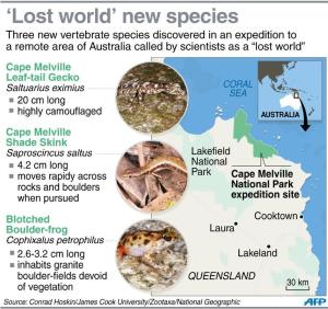
Figure 6. A-B shows a comparison of the distal cross-section of the Cryptoclidus femur (A; from
Brown, 1981)) to the profile of the NACA 6221 airfoil (B), the cross-section of the minke whale
foreflipper at the radius and ulna (C; from Cooper et al., 2008), and a cross-section of a cetacean
fluke (D; from Fish et al.; 2006). Soft tissue follows the contour of the minke whale foreflipper
until close to the trailing edge (C). The cetacean fluke is completely made up of soft tissue (D).
E-F shows a comparison of the planform shape of the minke whale foreflipper (E, from Cooper
et al.; 2008), penguin wing (F), and the hind flipper of Hydrorion brachypterygius (G; from von
Huene, 1923). A trailing edge made up of soft tissue extends posterior to the bones in all three
foils. Connective tissue makes up the trailing edge in the whale (E) while feathers make up the
trailing edge in the penguin (F).
DeBlois
29
29
The angle of attack (α) (Figure 4) also determines the value of lift and drag (Vogel,
1994). As α increases, so does lift reaching a maximum value (CLmax) at the critical angle of
attack (stall angle) (Vogel, 1994; Abbott and von Doenhoff, 1959). Past this angle, the flow
severely separates from the hydrofoil and lift goes down (Vogel, 1994; Webb, 1975; Fish and
Battle, 1995). Drag also tends to increase with α (after an initial reduction at low values of α)
and continues to increase past the stall angle (Vogel, 1994).
The aerodynamic forces of lift and drag depend on the complex interaction of the shape
of the hydrofoil (its camber, chord length, and thickness), the physical properties of the fluid
(density, velocity, and Reynolds number), and α (Abbott and von Doenhoff, 1959). For the
present study, fluid density and velocity are kept constant. The fluid is assumed to have steady
flow (stable velocity). Re is set to 10,000,000 (unless otherwise stated) as a simplification in
order to avoid the transition between laminar to turbulent flow, which occurs between 500,000
and 1,000,000 as well as reduce the effect of parasitic drag, which is predominant at Re <
500,000 (Vogel, 1994). A fixed value for Re is used since the length of the chord (c) is unknown
due to the missing trailing edge (which is presently being reconstructed).
METHOD
Inferring Flipper Shape from Fossil Specimens
The exact anatomy of the plesiosaur flipper is impossible to ascertain. However, the
cross-sectional and planform shape of the plesiosaur flipper form a clear hydrofoil shape even in
the absence of soft tissue (Figure 5, 6) (also see Wahl et al, 2010 and Carpenter, 2010). In
plesiosaurs and ichthyosaurs (an unrelated extinct marine reptile) the bony elements of the limbs
form a hydrofoil shape in planform (Taylor, 1987) and cross-section. Starting from the distal
DeBlois
30
30
end of the propodial (the root of the hydrofoil), the bones assume a hydrofoil shape in crosssection
(Figure 6). Undoubtedly, soft tissue surrounded the bones but it stands to reason that the
same hydrofoil shape is maintained even when surrounded by soft tissue. It is more
parsimonious for the limb to reflect the hydrofoil shaped bone that underlies it than for the bone
to evolve a hydrofoil shape only for that shape to be obscured by soft tissue. Assuming the bone
does reflect the shape of the functional hydrofoil, then the addition of soft tissue surrounding it
would only scale its size and not its shape.
Specimen. The following method for determining the functional flipper hydrofoil shape
was applied to the femur and humerus of Cryptoclidus eurymerus, HMG V1104 (figured in
Brown, 1981; presented again in Figure 9 below).
Image pre-processing. The cross-section of each propodial was obtained via end-on
distal view photographs. The resulting silhouette of the propodial at its widest section was taken
as the cross-sectional shape for that propodial. The photographs used were obtained directly or
indirectly through published photographs of the propodials. The fossil silhouettes were reduced
to single pixel outlines then converted to x,y-coordinates using the Pathfinder macro in ImageJ
(NIH ImageJ, Rasband 1997-2012). The outline was divided into the top and bottom curves
using the anterior-most and the posterior-most points as boundaries. The anterior end (fossil
leading edge) and posterior end (fossil trailing edge) of the outline were then examined for an
abrupt change in curvature as this signals the point at which the outline of the fossil bone no
longer traces the top or bottom surfaces of the hydrofoil. Coordinates past this point would not
contribute to the functional shape of the hydrofoil and were removed.
Estimating the leading edge. In order to recreate the rounded leading edge of the
hydrofoil, a circle was fitted to the anterior end of the propodial tangent to the lines connecting
DeBlois
31
31
the remaining two anterior-most coordinates each of the top and bottom curves. The arc of the
circle that extended anteriorly and connected the top and bottom curves was used in place of the
original anterior fossil outline. This substitution was necessary in order to correct for any wear
in the fossil or other breaks in the outline of the leading edge. The arc of the fitted circle usually
only slightly extended past the original fossil trailing edge.
Estimating the trailing edge. In contrast to the leading edge, the process of
approximating the size and shape of the trailing edge is comparatively more involved (Figure 8).
In order to parameterize the fossil outline and smooth out any irregularities, a polynomial was
fitted to the top and bottom surfaces separately. For this, I used the Class Shape Transformation
(CST) parameterization method specifically developed by Kulfan and Bussoletti (2006) (see also
Lane and Marshall, 2009) to formulate the polynomial that best fits a given set of points that
define an air/hydrofoil shape. This powerfully simple method could model a wide array of
shapes with a small number of equations and parameters (Kulfan and Bussoletti, 2006; Lane and
Marshall, 2009). The equations are the same as the Bezier curve equations with an added class
function term (equation 1 to 3 below) (Kulfan and Bussoletti, 2006; Lane and Marshall, 2009).
The class function term (equation 1 below) specifies a base or standard shape category from
which is derived all other shapes in that category (Kulfan and Bussoletti, 2006). This term also
reduces the number of coefficients necessary to parameterize the curve since the base shape that
is closest to the air/hydrofoil modeled could be chosen before the coefficients are set (Kulfan and
Bussoletti, 2006). The class function term is molded and transformed into the desired shape by
the shape function (equation 2 below), which is defined by a Bernstein Polynomial (Kulfan and
Bussoletti, 2006). The resulting fitted curves are smooth and do not suffer from the same degree
of oscillation problems that results from other parameterization methods such as B-Splines and
DeBlois
32
32
NURBS (Lane and Marshall, 2009). For a hydrofoil with a rounded leading edge and pointed
trailing edge, the class function,
!
C("),= is g"iv•en(1 b#y" )1
!
C(") = " (1#")1 (3)
where
!
" =
x
c
, x is the x-coordinate and c is the length of the chord of the hydrofoil (Figure 4).
The general form of the shape function,
!
S(") =
n!
r!(n # r)! r=0
n$
•"r • (1#"), is given by n #r
!
S(") =
n!
r!(n # r)! r=0
n$
Ar"r (1#")n #r (4)
where
!
S(") =
n!
r!(n # r)! r=0
n$
•"r • (1#")is the binomni#arl coefficient, n is the order of the Bernstein Polynomial, and
!
Stop (") = Atop,i
i=1
n#
• Sir is (")
the coefficient to be set using least-squares fitting. Combining the two equations yield the
general equation below for the function,
!
Z("), of a parameterized hydrofoil with a rounded
leading edge and pointed trailing edge
!
Z(") = " (1#")
n!
r!(n # r)! r=0
n$
Ar"r (1#")n #r (5)
For this study, a Bernstein Polynomial of order three (n = 3) was used for the top and bottom
curves since Bernstein Polynomials (n = 1 and 2) visibly fail to fit the outline of the fossil. The
DeBlois
33
33
expanded CST parameterization equation for a third order Bernstein Polynomial is given below
for the top curve
!
Z(")top = " (1#") A1(1#")3 + A2(1#")2" + A3(1#") "2 + A4"3 ( ) +"$ztop (6)
and the bottom curve
!
Z(")bottom = " (1#") A1(1#")3 + A2 (1#")2" + A3 (1#") "2 + A4"3 ( ) +"$zbottom (7)
where
!
"ztop =
zTE,top
c
is the thickness of the trailing edge tip for the top (
!
zTE,top ) normalized to the
length of the chord (Figure 4) and
!
"zbottom =
zTE,bottom
c
is the thickness of the trailing edge tip for
the bottom (
!
zTE,bottom ) also normalized to the length of the chord. For this study, the thickness of
the trailing edge tip was one pixel, thus a value of zero was used. The polynomial was fitted to
the points defining the fossil outline by determining the appropriate coefficients (A1 to A4) using
least-squares fit via the lsqnonlin command from the optimization toolbox in MATLAB.
In order to estimate the shape of a candidate trailing edge for the fossil outline, a point
was chosen posterior to the fossil to serve as the tip of the trailing edge (the point where the top
and bottom surfaces of the candidate trailing edge meet) (Figure 8). This point together with the
posterior end of the fossil forms a candidate trailing edge for the fossil hydrofoil. The
parameterized top and bottom curves were then interpolated to this point via shape-preserving
piecewise cubic Hermite interpolation (pchip) (Moler, 2004; Fritsch and Carlson, 1980). The top
and bottom curves were parameterized and interpolated separately then later recombined. This
DeBlois
34
34
interpolation was selected for its balance of smoothness and shape preservation (local
monotonicity). Full degree (global) interpolation does not preserve shape since it tends to vary
widely between points. On the other extreme, piecewise linear interpolation preserves shape but
lacks any smoothness. In between these two extremes are piecewise cubic spline interpolation
and shape-preserving cubic Hermite interpolation. Piecewise cubic spline interpolation
preserves shape better than full degree interpolation and is smoother than piecewise linear
interpolation but does not guarantee shape preservation (Moler, 2004). Indeed, piecewise cubic
spline interpolation tended to overshoot the y-value of the trailing edge tip within the gap
between the posterior-most edge of the fossil outline and the tip. On the other hand, shapepreserving
piecewise Hermite interpolation guarantees local monotonicity, which means that the
interpolated curve does not overshoot the trailing edge tip. However, it does so at the cost of
breaks in the second derivative (the first derivative is still continuous) whereas cubic spline
interpolation is continuous at the second derivative as well as the first. In other words, shapepreserving
cubic interpolation guarantees local monotonicity but is not as smooth as cubic spline
interpolation. For this study, shape-preserving piecewise cubic Hermite interpolation was
performed using the pchip option in the interp1 command in MATLAB.
At extreme trailing edge tips such as those too far posterior from the fossil outline, the
interpolated top and bottom trailing edge curves may intersect or overlap within the gap between
the fossil and the tip (Figure 8). Such instances produce hydrofoils that are beyond the
reasonable bounds of what is plausible biologically and reflect the limits of plausible shapes as
constrained by the top and bottom curvatures of the fossil outline. To circumvent this natural
limit and still evaluate the hydrofoil that would correspond to this trailing edge tip, I replaced
this trailing edge with the closest trailing edge whose tip falls along the same y-value (different
DeBlois
35
35
x-value) but that did not intersect or overlap. Prior to attachment, the replacement tip was
stretched along the x-axis such that it and the original tip being tested now have the same
endpoint x-value. The result was a mosaic hydrofoil with a stretched trailing edge (tail) that is
no longer fully constrained by the curvature of the top and bottom surfaces of the fossil. The
entire process from CST curve fitting through piecewise cubic interpolation and stretching was
performed through a custom MATLAB script that I generated (see Appendix 1).
The lift and drag of each complete hydrofoil (fossil outline + simulated trailing edge) was
determined using XFoil version 6.94, an airfoil simulation and design program (Drela, 1989;
Drela and Giles, 1987). XFoil models the flow streams around the hydrofoil and the wake using
a coupled viscous-inviscid panel method (Drela, 1989) given the following: the coordinate file
of hydrofoil, the Reynolds number (Re), Mach number (set to M=0), and Ncrit, which determines
where the transition laminar to turbulent flow transition occurs (set to
!
n˜ = 9). This method used
will only be briefly described here; for the detailed derivation see Drela and Giles (1987), Drela
(1989a, b), and Youngren (2001). In order to determine the flow around the hydrofoil, XFoil
divides the outline of the flipper and the wake into discrete panels (120 max), calculates the
potential flow around each panel, and then combines them to simulate the flow stream (Drela,
1989; Fearn, 2008). The flow around each panel is simulated using the superposition of the
freestream flow, a vortex distribution over the hydrofoil, and a source distribution over the
hydrofoil and wake. Altogether this forms a linear-vorticity streamfunction (Φ), given by
!
"(x, y) = u#y $ v#x +
1
2%
' & (s) lnr(s;x, y)ds + 1
2%
'( (s))(s;x, y)ds (8)
DeBlois
36
36
and
!
"(x, y) =
1
2#
% $ (s) lnr(s;x, y)ds + 1
2#
%& (s)'(s;x, y)ds (9)
where γ is the strength of the vortex distribution, σ is the strength of the source distribution, x,y
denotes a point on the flow field, s is a point along the panel, and r is the magnitude of the vector
between the points x,y and s with angle α;
!
u" (=
!
q" cos# ) and
!
v" (=
!
q" sin# ) are components
of the freestream velocity (
!
q"). The coefficient of pressure (CP) could then be approximated
from (8) and (9) using
!
Cp " #2
$ %
$x
q&
(10)
The coefficient of lift (CL) is directly calculated by integrating the pressure distribution around
the entire hydrofoil,
!
CL = Cp " dx (11)
where
!
x = x cos" + y sin" . The coefficient of drag (CD) is estimated by applying the Squire-
Young formula and evaluating the last point in the wake (≥ 1 chord length downstream):
!
CD = 2" (uedge /q#)(H +5) / 2 (12)
where uedge is the flow velocity at the edge of the boundary layer and H is the shape parameter.
DeBlois
37
37
In order to simulate viscous conditions, Xfoil address the inherent assumptions and
simplifications of the panel method, which is: the viscosity of the fluid is neglected, the flow
field has no vorticity, the flow is incompressible, and that the flow over the top and bottom
surfaces leave the trailing edge smoothly (Kutta condition) (Fearn, 2008). Fluid viscosity affects
the tendency of the flow to separate from the surface of the hydrofoil creating a boundary layer
of some thickness (θ). Flow about the hydrofoil now goes over the edge of this boundary layer,
effectively changing the shape of the hydrofoil. XFoil address this effect by applying the panel
method to the edge of boundary layer instead of the hydrofoil surface. It calculates the 2-
dimensional edge of the boundary layer using the following standard compressible integral
equations for the momentum thickness (boundary layer thickness, θ) and kinetic energy shape
parameter (H*):
!
d"
d#
+ 2 + H $ Medge ( ) "
uedge
duedge
d#
=
Cf
2
(13)
!
"
dH*
d#
+ (2H** + H*(1$ H)) "
uedge
duedge
d#
= 2Cdissipation $ H* Cf
2
(14)
where ξ is the boundary layer coordinate, Medge is the Mach number at the edge of the boundary
layer (Medge = 0 throughout this study), uedge is the velocity at the edge of the boundary layer, Cf
is the skin-friction coefficient, Cdissipation is the dissipation coefficient, H is the shape parameter,
and H** is the density shape parameter. The following dependencies in functional notation are
assumed in order to evaluate equations (13) and (14):
DeBlois
38
38
H* = H*(Hk, Medge, Reθ ) (15)
H** = H**(Hk, Medge ) (16)
Cf = Cf (Hk, Medge, Reθ ) (17)
CD = CD (Hk, Medge, Reθ ) (18)
where Reθ is the Reynolds number multiplied by the boundary layer thickness (θ). The specific
expressions are given in Drela and Giles (1987). Another simplification inherent to the panel
method is that the flow field does not have any vorticity (the curl of the velocity field is assumed
to be zero). Turbulent flow affects the thickness of the boundary layer differently from laminar
flow. XFoil address this by calculating the above dependencies (15, 16, 17, 18) for laminar and
turbulent flows then switching from between those expressions at the transition point. In order to
do so, XFoil determines where this transition occurs by modeling the growth of the amplitude of
the largest Tollmien-Schlichting wave (
!
n˜ ) using the equation below:
!
dn˜
d"
=
dn˜
dRe#
(Hk )
dRe#
d"
(Hk ,# ) (19)
The transition is assumed to occur when the preset value for
!
n˜ is met. In the present study, the
standard value of
!
n˜ = 9 is used throughout. To account for the compressibility of flow, XFoil
uses the Karman-Tsien correction, which depends on the Mach number. However, for the
present study, the Mach number is set to zero (M = 0) so this correction does not apply and the
assumptions is made that the flow is incompressible. Since the fluid medium for the present
study is water (essentially incompressible under normal conditions) and the flow speed is low,
DeBlois
39
39
this is a valid assumption. Finally, XFoil assumes that the flow over the top and bottom surfaces
leaves the trailing edges moothly (Kutta condition).
XFoil calculates the solution to the streamfunction and boundary conditions using the
linear algebra and the Newton-Raphson method (Drela and Giles, 1987; Drela, 1989). Starting
with an estimate of the value of the solution, successive iterations are made using solutions from
the preceding iteration until the answer is obtained by convergence or until the maximum
number of iterations is reached. For the present study, the maximum number of iterations is set
to 300. If XFoil fails to converge to an answer, a L/D value of zero is assigned to that airfoil.
A set of complete hydrofoil shapes (fossil outline + candidate trailing edge) with different
trailing edge shapes were evaluated using XFoil. The trailing edge tip was used to determine the
shape of the trailing edge via interpolation from the posterior end of the fossil outline (see
above). The location of the trailing edge tip is determined by sampling the x,y-coordinate space
posterior to the fossil at coarse (5% of the cross-sectional length of the fossil element) and fine
intervals (1% of cross-sectional length) (Figure 9). The x,y-coordinate of the leading edge of the
fossil outline is set to (0,0) and the rest of the fossil element is scaled to span the x-coordinates
from 0 to 1. The L/D ratio is obtained using XFoil for each completed hydrofoil shape (fossil
outline + candidate trailing edge) at various angles of attack (usually from -10º to +10º at 0.25º
increments). This range is usually sufficient to determine the angle of attack with the maximum
L/D. A Re value of 10,000,000 is used to test the hydrofoil shapes. This Re value is within the
range of Re experienced by cetaceans, large marine animals comparable to plesiosaurs (Fish,
1993). This value was chosen in order to avoid the transition from laminar to turbulent flow
which would occur at Re between 500,000 and 1,000,000. The sign of L/D depends on which
side has the lower pressure (dorsal or ventral side of the hydrofoil) with the dorsal side given a
DeBlois
40
40
positive (+) sign and the ventral side given a negative (-) sign. The L/D value for each candidate
hydrofoil is plotted on the z-axis with the x,y-coordinate of the corresponding trailing edge tip
plotted on the x,y-plane. This produces a 3-D contour plot of the sample space for a particular
angle of attack. The largest lift-to-drag ratio (L/D) for the complete hydrofoil (fossil outline +
candidate trailing edge) was used as criterion to determine the best functional trailing edge for
the fossil element among the set of candidates.
Figure 7. The skeletal reconstruction of Cryptoclidus eurymerus is shown in A (from Brown,
1981). The planform of the fore flipper (from Storrs, 1993) and hind flipper (modified from
Andrews, 1913) are shown from left to right, respectively, in B. The humerus and femur (from
Brown, 1981) are shown from left to right, respectively, in C. The distal cross-section of the
femur and humerus (from Brown, 1981) are shown from left to right, respectively, in D. Both
scale bars are 5 cm. Note how the humerus angles forward from the base (B) and how rest of the
flipper from the radius and ulna makes a sharp angle backward.
DeBlois
41
41
Figure 8. Flow chart of the steps involved in creating the shape for the complete hydrofoil.
Briefly, (from the left column top to bottom) the outline of the surface of the hydrofoil (in red) is
parameterized by curve-fitting (in blue). A point is selected posterior to the fossil outline to
serve as the trailing edge tip. The fossil outline is then interpolated to this point filling the gap in
between (in cyan) and the hydrofoil is constructed. If the interpolation results in the top and
bottom curves crossing within this gap (center of the middle column), the trailing edge is
removed and replaced with the closest trailing edge with the same x-coordinate that did not
cross. This trailing edge is then stretched such that the stretched tip reaches the desired trailing
edge tip (last column, in magenta).
DeBlois
42
42
Figure 9. Sample contour plot showing the position of the trailing edge tips and corresponding
L/D values. The x,y-coordinate plane posterior to the fossil element, in this case, the femur of
Cryptoclidus eurymerus (A) from Brown (1981) was sampled for the location of the trailing edge
tip that, together with the fossil outline, would produce the functionally best performing
hydrofoil shape. For coarse sampling the points are spaced apart by 5% of the length of the
fossil. For fine sampling this space is reduced to 1% of the length of the fossil. Shown in (B) is
the resulting contour plot at angle of attack (α) of 2.25º. The L/D obtained through XFoil for
each hydrofoil is plotted with the x,y-coordinate of the tip on the x,y-plane. Cool colors denote
high magnitude lift generated from the dorsal side (positive L/D), termed “dorsal lift”. Hot
colors denote high magnitude lift generated from the ventral side (negative L/D ratio), termed
“ventral lift”.
DeBlois
43
43
RESULTS
C. eurymerus Femur Hydrofoil
The 2-D functional hydrofoil shape was reconstructed for the distal cross-section of the
C. eurymerus femur from specimen HMG V1104, figured in Brown (1981) (Figure 7). The
contour plots for the set of candidate hydrofoil shapes for the femur is shown in Figure 10 for the
range of angle of attack (α) from -8º to +8º. The plots shown here is only a subset of the full
range of angles of attack examined (α from -10º to +10º at 0.25º increments). Highlighted in
magenta in Figure 10 are the shapes with L/D (= CL/CD) values within the top 5%. This region
of high positive L/D values (positive because lower pressure is on the dorsal side of the
hydrofoil) first appears around 0º, peaks by +2º, and disappears again by +4º (Figure 10, Table
2). At α below +2º the ventral side of the hydrofoil produces lift and a negative L/D value is
obtained. Highlighted in red in Figure 10 are the shapes with L/D values within the bottom 5%.
The peak range of ventral directed lift (“ventral lift”) is attained by α = -2º (max L/D = -126),
which persists and expands beyond α = -8º. Indeed, this plateau persists past α = -10º and only
starts to wane past α = -15º. This is in stark contrast to the relatively short-lived but high
magnitude “dorsal lift” (max L/D = 308).
The reconstructed hydrofoil shape of the C. eurymerus femur is shown in Figure 11. This
hydrofoil shape is among the shapes that most consistently produced L/D values in the top 5%
across the range of α where the top 5% L/D values occur (α = -0.75º to 3.75º). Additionally, the
x,y-coordinate of its trailing edge tip is the spacial mean of the x,y-coordinates of the trailing
edge tips of these hydrofoils. The reconstructed trailing edge comprises about 26% of the overall
hydrofoil shape based on the x-coordinate of the trailing edge tip (Figure 11, Table 2). This
produces a chord length of about 0.24 m and a maximum camber of about 11% (relative to chord
DeBlois
44
44
length) located at 36% of the chord length from the leading edge (Figure 11, Table 2). The
corresponding plots of CL vs α, CD vs α, and L/D vs α for the reconstructed hydrofoil shape are
shown in Figure 11 (B-D respectively). Their values are obtained through XFoil. The Re used
was calculated using Equation 1 (see above) from the chord length of the reconstructed hydrofoil
shape and assuming a flow velocity of 1 m/s (the swim speed estimate by Motani, 2002).
Together with the kinematic viscosity of water (η = 1.0x10⁻⁶ m2/s), the Re value used was
240,000. The highest value of lift (CLmax) obtained at this Re value is 2.02 at α = 26.75º (Figure
11, Table 2). This α is also known as the stall angle since the value of CL drops drastically past
this α. The lowest value of drag (CDmin) is 0.042 and occurs at -11.75º (Figure 11, Table 2). The
maximum value of the lift to drag ratio (max L/D) is 16.52 and occurs at α = 13.25º.
C. eurymerus Humerus Hydrofoil
The 2-D functional hydrofoil shape was reconstructed for the distal cross section of the
C. eurymerus humerus from specimen HMG V1104, figured in Brown (1981) (Figure 7). The
contour plots obtained for the set of candidate hydrofoil shapes for the C. eurymerus humerus is
shown in Figure 12 for α from -8º to +8º. As with the femur, the range of α shown here is only a
subset of the full range examined (-10º to +10º at 0.25º increments). (These contours are
stacked, in order, to form a movie, see Supplemental Figure S2). The top and bottom 5% are
highlighted in magenta and red respectively. The top 5% L/D values are centered around α = 0º
with a the highest value at α = 0.75º (max L/D = 223). The bottom 5% appears around α = -4º,
peaks at α = -8º (max L/D = -134) and continues past α = -10º.
DeBlois
45
45
Figure 10. Contour plots for the C. eurymerus femur for α from -8º to +8º. The x,y-coordinates
of the trailing edge tip is plotted on the x,y-plane with the magnitude of the L/D resulting from
the corresponding completed hydrofoil (trailing edge + fossil outline) plotted as contours. Cool
colors denote dorsal oriented lift (max L/D = 308) and hot colors denote ventral oriented lift
(max L/D = -126). In magenta are the shapes with L/D values within the top 5%. In red are the
shapes with L/D values within the bottom 5%.
DeBlois
46
46
Figure 11. The reconstructed hydrofoil shape for the C. eurymerus femur (A). Shown in B-D,
respectively, are the plots of CL vs α, CD vs α, and L/D vs α using Re = 240,000.
Scale bar = 5 cm.
Stall angle
CLmax
DeBlois
47
47
Figure 12. The contour plots for the C. eurymerus humerus for α from -8º to +8º, plotted as in
Figure 10. Cool colors denote dorsal oriented lift (max L/D = 223) and hot colors denote ventral
oriented lift (max L/D = -136). In magenta are the shapes with L/D values within the top 5%. In
red are the shapes with L/D values within the bottom 5%.
DeBlois
48
48
Figure 13. The reconstructed hydrofoil shape for the C. eurymerus humerus is shown in A.
Shown in B-D, respectively, are the plots of CL vs α, CD vs α, and L/D vs α using Re = 390,000.
Scale bar = 5 cm.
The reconstructed hydrofoil shape of the C. eurymerus humerus is shown in Figure 13.
This hydrofoil shapes is among those that most consistently produced L/D values in the top 5%
across the range of α where the top 5% occur (-1.75º to 1.75º). Its trailing edge tip x,ycoordinate
also corresponds to the spacial mean of the x,y-coordinates of these hydrofoils. The
reconstructed trailing edge soft tissue for the humerus comprises about 43% of the entire
hydrofoil shape based on the x-coordinate of the trailing edge tip (Figure 13, Table 2). This
DeBlois
49
49
produces a chord length of about 0.39 m and a maximum camber of 11% (relative to chord
length) located at 54% of the chord length from the leading edge (Figure 13, Table 2). The
corresponding plots of CL vs α, CD vs α, and L/D vs α for the reconstructed hydrofoil shape are
shown in Figure 13 (B-D respectively). The Re (= 390,000) used was calculated from the chord
length of the reconstructed hydrofoil shape and assuming a flow velocity of 1 m/s (Motani,
2002). At this Re, the reconstructed humerus hydrofoil attains CLmax = 1.95 at α = 20.5, CDmin =
0.013 at α = -2.5º, and max L/D = 78.0 at α = 4.15º (Figure 13, Table 2).
In order to further characterize the hydrodynamic properties of the reconstructed
hydrofoils, they were compared to engineered hydrofoils that have similar shapes, the Wortmann
FX 63-137 (Althaus and Wortmann, 1981) and NACA 63(3)-618 (Figure 14, Table 2). Since the
original Wortmann FX 63-137 airfoil coordinates were not analytically smooth (Selig and
McGranahan, 2004), the airfoil coordinates used in this study are those that have been previously
smoothed out (Selig and McGranahan, 2004). The C. eurymerus humerus hydrofoil and the
Wortmann FX 63-137 airfoil have similar maximum thickness, location of maximum thickness,
and location of maximum camber (Figure 14, Table 2). However, the maximum camber for the
humerus hydrofoil is 11% while for the Wortmann FX 63-137 airfoil it is only 6% (Figure 14,
Table 2). Under the same Re (= 390,000), both foils attained similar values for CLmax, CDmin, and
stall angle (Table 2). However, the Wortmann FX 63-137 airfoil has a larger maximum L/D
value (115.8 vs 78.0 for the humerus hydrofoil; see Table 2).
The NACA 63(3)-618 airfoil and C. eurymerus femur hydrofoil have similar maximum
thickness and location of maximum thickness (Table 2). However, the femur hydrofoil has a
larger maximum camber (11% vs 3% for the NACA 63(3)-618) airfoil that is located further
back (63% vs 50% for the NACA 63(3)-618). Under the same Re (= 240,000), the femur
DeBlois
50
50
hydrofoil attained higher CLmax and CDmin values but lower maximum L/D compared to the
NACA 63(3)-618 airfoil. The stall angle for the femur hydrofoil is slightly larger at 26.75º
compared to 20.5º for the NACA 63(3)-618 airfoil.
The reconstructed C. eurymerus hydrofoils were also compared to published values of CL
at α = 10º under inviscid conditions (Table 3) for various cetacean taxa (Fish et al., 2007) as well
as the Wortmann FX 63-137 airfol, the NACA 63(3)-618 airfoil, and the NACA 0021 airfoil,
which has no camber and, thus, is symmetric about the chord. The C. eurymerus hydrofoils and
the similarly shaped engineered hydrofoils (Wortmann FX 63-137 airfol and the NACA 63(3)-
618 airfoil) had noticeably higher CL values (Table 3) compared to the cetacean fluke hydrofoils
and the NACA 0021 airfoil.
Figure 14. The reconstructed C. eurymerus humerus and femur hydrofoils with similarly shaped
engineered airfoils. Scale bar = 5 cm.
DeBlois
51
51
Table 2: Geometric and hydrodynamic properties of the C. eurymerus femur and humerus
compared to engineered airfoils with matched Re.
C. eurymerus
Humerus
C. eurymerus
Femur
Wortmann
FX 63-137
NACA
63(3)-618
% soft tissue (based on x-value of
trailing edge tip)
43% 26% - -
Chord length ~ 0.39 m ~ 0.24 m - -
Max camber (% chord length) 11% 11% 6% 3.3%
Location of max camber (% chord
length)
54% 63% 57% 50%
Max thickness (% chord length) 13% 22% 14% 18%
Location of max thickness (%
chord length)
29% 36% 31% 35%
Re 390,000 240,000 390,000 240,000
CLmax 1.95 2.02 1.82 1.44
CDmin 0.013 0.042 0.009 0.013
Max L / D 78.0 16.5 115.8 79.8
Stall angle 20.5º 26.75º 19.75º 20.5º
Table 3: Inviscid comparison of lift coefficient (CL) at α = 10º among the C. eurymerus
hydrofoils, cetacean flukes from various taxa taken at rest (from Fish et al., 2007), and
engineered airfoils with (NACA 63(3)-618 and Wortmann FX 63-137) and without camber
(NACA 0021).
Species / Designation Hydrofoil element cross-section CL
Cryptoclidus eurymerus Distal cross-section of humerus 2.57
Cryptoclidus eurymerus Distal cross-section of femur 2.77
Delphinus delphis Cross-section at 50% of fluke span 1.16
Globicephala malaena Cross-section at 50% of fluke span 1.27
Grampus griseus Cross-section at 50% of fluke span 1.32
Kogia breviceps Cross-section at 50% of fluke span 1.26
Lagenorhynchus acutus Cross-section at 50% of fluke span 1.33
Phocoena phocoena Cross-section at 50% of fluke span 1.29
Stenella sp. Cross-section at 50% of fluke span 1.31
Tursiops truncatus Cross-section at 50% of fluke span 1.34
NACA 0021 - 1.29
NACA 63(3)-618 - 1.82
Wortmann FX 63-137 - 2.24
DeBlois
52
52
DISCUSSION
The method described here is the first to quantitatively reconstruct the trailing edge soft
tissue and resulting functional shape of the plesiosaur flipper (Figure 11, 13, and 16). This
enables, for the first time, the quantification of the hydrodynamic properties of plesiosaur
flippers. This method was applied to the distal cross-section of the C. eurymerus humerus and
femur resulting in the reconstructions shown in Figure 11 for the femur and Figure 14 for the
humerus. Now that the functional shape of the flipper is complete, the chord length, camber, and
thickness distribution of the flipper could be obtained and used to assess the hydrodynamic
properties, such as lift and drag, that emerge from the hydrofoil geometry (Table 2).
The hydrodynamic properties of the reconstructed humerus and femur hydrofoils were
assessed using XFoil and a Re value calculated using equation 1 from the chord length of each
hydrofoil respectively, a flow velocity of 1 m/s based on estimates of optimal swimming speed
for Cryptoclidus by Motani (2002), and the kinematic viscosity of water (Table 2). At these
respective Re values, the reconstructed hydrofoils for the humerus and femur have similar values
of CLmax (~ 2, see Table 2). However, the humerus hydrofoil has a lower value of CDmin than the
femur hydrofoil (0.013 compared to 0.042, respectively; Table 2) due in part to the lower
thickness of the humerus. This results in a higher maximum L/D ratio for the humerus hydrofoil
(78.0 compared to 16.5, respectively; Table 2). Interestingly, the reconstructed humerus and the
femur hydrofoils have very similar maximum camber (11%, relative to chord length; Table 2).
This relatively high camber endows the C. eurymerus hydrofoils with high CLmax values and
large stall angles (Table 2 and 3). The CLmax values for the C. eurymerus hydrofoils are
noticeably greater than those for cetacean fluke hydrofoils taken at rest, which has little to no
camber (Table 3) (Fish et al., 2006; 2007). The NACA 0021 airfoil, which has zero camber,
DeBlois
53
53
produces a CLmax value within the range of values for the cetacean fluke hydrofoils while the
cambered Wortmann FX 63-137 and NACA 63(3)-618 airfoils fall in the same range of values as
the C. eurymerus hydrofoils (Table 3). When compared side-by-side, the C. eurymerus humerus
has modestly greater camber than the similarly shaped Wortmann FX 63-137 airfoil.
Consequently, under the same Re value (390,000) the humerus hydrofoil and the Wortmann FX
63-137 airfoil have similar CLmax values and stall angles (1.95 vs 1.82 and 20.5º vs 19.75º
respectively; Table 2). The difference in camber is greater between the C. eurymerus femur
hydrofoil and the similarly shaped NACA 63(3)-618 airfoil (11% vs 3% relative to chord length;
Table 2). Consequently compared to the NACA 63(3)-618 airfoil, the femur hydrofoil has
greater CLmax (2.02 vs 1.44) and greater stall angle (26.75º vs 20.5º) under the same Re value
(240,000; see Table 2). However, the maximum L/D ratio is greater for the Wortmann FX 63-
137 and the NACA 63(3)-618 airfoil than for the C. eurymerus humerus and femur hydrofoils,
respectively, due to the lower CDmin values attained by the engineered airfoils.
Cryptoclidus eurymerus was a slow but maneuverable swimmer. The hydrodynamic
properties of the reconstructed hydrofoils for the distal cross-section of the humerus and femur
for C. eurymerus presented in this study suggest that the fore and hind flippers are adapted for
slow swimming with high maneuverability. The most prominent feature of both hydrofoils is the
high degree of camber, which results in high CLmax values and high stall angles. This prevents
the loss of lift (and hence thrust) at slow speeds resulting in greater maneuverability. The
rearward position of maximum camber (past 50% of chord length; see Table 2) further aids
maneuverability by reducing the drop in CL immediately following the stall angle (Abbott and
von Doenhoff, 1959). The planform shape of the flippers (Figure 7) further supports a slow, but
maneuverable specialization for the flippers. Reconstructed in Figure 15 is the planform shape
DeBlois
54
54
of the fore flipper and hind flipper incorporating the reconstructed hydrofoil cross-sections of the
humerus and femur, respectively. The fore and hind flippers both have low aspect ratios (ARs),
based on the skeletal elements of the flippers alone (O’Keefe, 2001b). When combined with the
reconstructed trailing edges at the distal tip of the humerus and femur, the planform shape
becomes even broader further reducing the AR (Figure 15). Low AR hydrofoils are not as
efficient as those with high AR (ratio of CL/CD is smaller) but, in exchange, enable slower speeds
and higher maneuverability (Vogel, 1994), a trend observed in birds (O’Keefe, 2001b) and
cetaceans (Woodward et al., 2006; Fish 2004). Part of the reduction in efficiency is the larger
value of CD due to greater induced drag (Vogel, 1994). This is reduced by a distally tapering
planform and by having a sweepback (Kucherman, 1953; Ashenberg and Weihs, 1984). These
are both features of the fore and hind flippers of C. eurymerus (Figure 7, 15). Importantly, the
degree of taper is pronounced in the fore flipper and the sweepback is strongly exaggerated
(Figure 7, 15). The humerus extends anteriorly, unlike in any other plesiosaur, and from there,
the rest of the flipper starting with the radius and ulna angles posteriorly (Figure 7, 15).
Altogether, the C. eurymerus flippers enable slow swimming speeds and greater maneuverability
based on a high CLmax value, a high stall angle (Table 2), and a low AR planform coupled to a
distally tapering planform with pronounced sweepback that reduces drag.
DeBlois
55
55
Figure 15. Planform reconstruction of the fore flipper and hind flipper of Cryptoclidus
eurymerus (on the left and right, respectively). In blue is the outline of the planform made by
connecting the tip of the reconstructed trailing edge at the distal end of the propodial to the tip of
the phalanges. In red is the outline of another possible planform. The more cross-sectional
hydrofoil shapes are reconstructed, the better the resolution of the shape of the flipper will be.
The skeletal reconstruction of the flipper planform is from Storrs (1993) for the fore flipper and
Andrews (1910) for the hind flipper. Scale bar = 5 cm.
Although the exact anatomy of the plesiosaur flipper is impossible to ascertain, the
functional shape of the plesiosaur flipper is approximated using the quantitative method
presented here with only a few assumptions and simplifications. The first assumption is that the
shape of the fossil element closely matches the functional shape of the flipper with soft tissue
intact. As Figure 6 illustrates in extant animals, the bones that make up the flipper (Figure 6c) is
responsible for the cross-sectional hydrofoil shape. The soft tissue that surrounds the bone
DeBlois
56
56
follows its curvature such that the shape formed by the outline of the bones is reflected in the
shape of the functional hydrofoil. Soft tissue increases the overall size of the hydrofoil but does
not obscure the shape formed by the bones. Therefore, it is reasonable to use the outline of the
fossil bones to derive the functional shape of the flipper.
Another assumption is that the best functioning hydrofoil (top 5% L/D) would also be a
likely shape for the plesiosaur flipper hydrofoil. This assumption was used as the basis for
constraining the set of possible hydrofoil shapes for the fossil element from the thousands tested
by the method. Webber and colleagues (2009) compared idealized physical representations of
several cetacean flipper hydrofoils and compared their hydrodynamic properties to real,
anatomical flippers. They found the idealized flippers to underestimate the CD value of the real
flipper they were supposed to mimic. Likewise, the true plesiosaur flipper was likely to be suboptimal.
However, identifying the degree to which the flipper of an extinct animal is suboptimal
is extremely difficult, if not impossible. Using best performance as criterion is more
manageable and easier to apply and also sets the limit on what is possible.
Steady flow is also assumed. The performance of the hydrofoil shapes were analyzed
and compared to one another under steady flow. In an actively swimming animal the direction
and magnitude of flow around the flippers would change during the stroke cycle. However,
whether or not the flow around the flipper could be accurately simplified as steady or unsteady
could be calculated and is given by the aerodynamic frequency parameter (also known as the
reduced frequency value), ω, which is a measure of the unsteady effects of flow about the
hydrofoil:
ω = 2πƒc/U (20)
DeBlois
57
57
where ƒ is the wingbeat frequency, c is the chord of the hydrofoil (Figure 4), and U is the
velocity of the flow. For dolphins, ω > 0.5 (Fish 1993), which suggests that the steady flow
around the flippers cannot be assumed. The same is likely to be also true for plesiosaurs.
However, the method does not aim to determine the kinematics of the plesiosaur flipper during
the stroke cycle. Steady flow is used only to characterize the hydrodynamic properties of the
shapes in order to identify the best functional hydrofoil shape for the fossil element.
The L/D ratio of the candidate hydrofoils for Re = 10,000,00 is used to determine the best
performing hydrofoil shape. This relatively high Re value was chosen in order to bypass the
transition from laminar to turbulent flow, which occurs between 500,000 and 1,000,000, and
simplify the behavior of the flowstream. This is within the range of Re experienced by the body
of swimming dolphins as a whole (Fish, 1993) and is likely within the range of Re experienced
by the body of plesiosaurs as a whole as well (mentioned in Motani, 2002). However, the shorter
length of the flipper cross-section compared to the whole animal would mean that the Re
experienced by the hydrofoil would be smaller. That is, unless the velocity of the flipper motion
makes up for the smaller length of the flipper during the stroke cycle by being proportionally
higher than the velocity of the animal (see equation 1). However, consideration of the
kinematics of the stroke cycle is beyond the scope of XFoil and, hence, the method used here.
Since the length of the functional flipper changes with every hydrofoil shape candidate, the Re
was kept constant and instead the speed of the flow about the hydrofoil was allowed to change
(see equation 1). Alternatively, the speed could have been kept constant that the Re calculated
for each hydrofoil shape. However, doing so would entail considerable additional programming
DeBlois
58
58
since the Re value would have to be calculated for each hydrofoil shape and its input into XFoil
for each of the thousands of hydrofoil shapes would have to be automatized.
Lastly, the assumptions and simplifications inherent to using XFoil also apply to the
present method. The values of CL and CD are obtained by calculating and applying potential
flow over a mathematically determined boundary layer and laminar-to-turbulent transition.
XFoil is sufficient to obtain a rough estimate of the hydrodynamic properties of the hydrofoil
shapes in order to obtain the functionally best performing shape. Subsequent in-depth
investigations and characterizations of the hydrofoil shape should be reserved for more
sophisticated programs and, ideally, flow tank experiments using physical models.
The method introduced in this study is the first to quantitatively reconstruct the crosssectional
shape of the plesiosaur flipper hydrofoil. It was used to reconstruct the trailing edge
soft and resulting hydrofoil shape of the distal propodial of the plesiosaur C. eurymerus.
However, it could just as easily have been applied to any cross-section along the length of the
flipper assuming the shape of the fossil elements is intact and separate elements properly
articulated. Furthermore, this method is not limited to plesiosaur flippers but could also be
applied to approximate the shapes and hydrodynamic properties of flippers from other extinct
taxa like ichthyosaurs.
DeBlois
59
59
CHAPTER 3: FUTURE WORK – VALIDATION EXPERIMENTS
INTRODUCTION
A few assumptions and simplifications were made in the method introduced in this study
in order to address the problem of reconstructing the soft tissue that forms the trailing edge of the
plesiosaur flipper. One is that the best functional hydrofoil shape closely approximates the shape
of the real plesiosaur hydrofoil. The other is that the best functional hydrofoil shape would be
the same no matter the Reynolds number (Re) used. The first is addressed by taking a crosssection
of a hydrofoil from an extant animal such as the fluke and flipper hydrofoils of whales
and the wing of a penguin, removing some portion of the trailing edge, then comparing the best
functional shape obtained with the method to the full cross-section of the flipper. The second is
addressed by using different Re values to determine the best functional shape of the hydrofoil for
the same fossil element, e. g. the Cryptoclidus eurymerus femur.
METHOD
In Part 1, the same method introduced in Chapter 2 is used here to determine the
functional shape of truncated whale fluke and penguin wing hydrofoils. In Part 2, the same
method as in Chapter 2 will be used and once again applied to the C. eurymerus femur except the
Re number will be varied.
DeBlois
60
60
PRELIMINARY DATA
The contour plots for C. eurymerus femur corresponding to Re of 107, 106, 500,000 and
250,000 are shown in Figure 16.
Figure 16. Contour plots for the C. eurymerus femur at Re = 10,000,000; Re = 1,000,000; Re =
500,000; and Re = 250,000 for α between -2º and +10º.
INTERPRETATION
Reducing the Re increases the angle of attack (α) at which the highest L/D ratio occurs
(Figure 16). The general topography stays the same however and no noticeable differences
occur in the x,y-coordinate location of the trailing edge tip that produces a hydrofoil shape with
the highest L/D ratio. An in-depth analysis should be performed in order to ascertain that
changing Re has minimal effect on the shape of the best performing hydrofoil.
DeBlois
61
61
CHAPTER 4: FUTURE WORK – PLESIOSAUR FLIPPER
KINEMATIC HYPOTHESIS
INTRODUCTION
A few assumptions and simplifications were made in the methods that preclude a
kinematic analysis of the plesiosaur flipper, specifically the steady flow assumption. However,
without losing sight of this caveat, it is possible to use the method presented here to develop a
kinematic hypothesis for the plesiosaur stroke cycle. This hypothesis could then be tested more
rigorously with the appropriate program simulator or flow tank experiments with physical
models. The logic is that the most effective angles of attack (α) would reflect changes in the
direction of flow that occur during the stroke cycle. The best α could be interpreted as the
dominant angle of attack and the lower and upper bounds of the most effective α could be
interpreted as the limits of range of motion. Additionally, since the shape of plesiosaur flipper
hydrofoil would be changing during the stroke cycle as α changes (Figure 17), one could then
take the best performing shapes (highest L/D) for each α and reconstruct the shape changes that
occur during the stroke cycle. I present one such hypothesis for the kinematics of the
Cryptoclidus eurymerus hind flipper here, at the level of the femur.
METHOD
From the set of candidate C. eurymerus femur hydrofoils obtained in the study in Chapter
2, a subset is created comprised of the best performing hydrofoil shape and the other hydrofoil
shapes that have the same mean line length. The mean line follows the curvature of the hydrofoil
and so would be a good indicator of flipper length. From this subset, the best performing shape
DeBlois
62
62
is determined for each α. The shapes are then placed in order based on α to reconstruct the full
range of changes that accompany the stroke cycle. Consideration is given to the α that produces
the highest L/D as this likely dominates the stroke cycle.
PRELIMINARY DATA
For the C. eurymerus femur, the best performing hydrofoil shape (assuming steady flow
with no turbulence and a relatively high Reynolds number) is shown in Figure 11 and again in
Figure 17. The trailing edge that corresponds to this shape is in black. The cyan-colored trailing
edges are other trailing edge shapes that did not perform as well as the one in black but have the
same length (measured via the mean of the top and bottom surface coordinates, within ±2.5% of
the length of the best performing hydrofoil). Since the trailing edge is made up of soft tissue and
likely to be flexible, these auxiliary shapes might be different forms of the same trailing edge.
DeBlois
63
63
Figure 17. Shown in (A) is the best functional hydrofoil shape for the Cryptoclidus eurymerus
femur (in black) superimposed on top of the other hydrofoil shapes that have the same mean line
length (in cyan). These shapes are hypothesized to be the shapes the hydrofoil shapes that arise
during the stroke cycle as the trailing edge soft tissue deflects/moves up and down. In (B) is
plotted the highest L/D values at Re = 10,000,000 for the hydrofoil shapes that have the same
mean line length as the best functional hydrofoil.
INTERPRETATION
The changes in shape of the hydrofoil trailing edge at corresponding angles of attack
reflect the kinematics of the femur stroke cycle. The femur is more effective at producing a
dorsally oriented lift vector (Figure 17), which coincides with the asymmetric, dorsally oriented
DeBlois
64
64
camber of the fossil cross-section (not including the trailing edge). This means that for the
power stroke the dorsal side of the flipper must have a forward directed component with respect
to the animal. This is achieved parsimoniously in a forward-moving animal only if the dorsal
side of the flipper is tilted forward in addition to a downward movement of the hydrofoil; only
then will the net flow locally around the hydrofoil have a rearward and upward orientation that
together with the forward tilt of the hydrofoil produces a forward directed lift component.
Upward movement of the hydrofoil would orient the dorsal side of the hydrofoil backward and
would lead to a rearward facing lift component. Therefore, the power stroke must be the
downstroke. Furthermore, the most effective angle of attack (highest L/D magnitude) is around
0º, which coincides with a forward tilted hydrofoil facing a rearward and upward flow stream.
This angle of attack and corresponding trailing edge shape likely dominates the downstroke. As
the angle of attack increases to +4º (Figures 17) the orientation of the trailing edge switches from
ventral to dorsal, which in turn changes the curvature of the hydrofoil from having dorsally
oriented camber (convex side up) to having ventrally oriented camber (convex side down). The
top and bottom flow streams separate beyond +4º, which suggests that the transition from
positive to negative angles of attack occurs at +4º. This signals the transition from one stroke to
the other, from downstroke to upstroke. The switch in sign of the L/D value at -5.25º marks the
other stroke transition, from upstroke to downstroke. At the start of the upstroke, the angle of
attack is shallower than at the downstroke, around -10º. A shift in angle of attack in the negative
direction would result if the magnitude of the rearward flow stream is much larger than the
downward flow stream (upward motion of the flipper). Since the hydrofoil now has a ventral
camber (convex side down) and consequently the lift vector is oriented toward the ventral side of
the hydrofoil, upward movement continues to produce a forward oriented lift component,
DeBlois
65
65
although not as much as in the downstroke. Towards the end of the upstroke, the angle of attack
approaches -5º. At the end of the upstroke the trailing edge flips back to the ventral side (convex
side up) and the hydrofoil tilts sharply to a downward orientation with an angle of attack of -5º.
Altogether, the swimming motion of the femur is as follows: at the start of the downstroke, the
hydrofoil is angled sharply downward with an angle of attack around -5º; the hydrofoil then tilts
quickly to an angle of attack around 0º and maintains this angle for most of the downstroke;
towards the bottom of the stroke, the hydrofoil tilts further up to an angle of attack at +4º at the
bottom; at the same time, the trailing edge of the hydrofoil transitions from curving ventrally
(convex side up) to curving dorsally (convex side down); this marks the end of the downstroke
and the start of the upstroke; at this point the flipper is cambered ventrally (convex side down);
the magnitude of the velocity of the upstroke is not as large as the downstroke, consequently the
hydrofoil has a shallower upstroke angle of attack; towards the end of the upstroke, the angle of
attack sharpens to -5º before reaching the end of the upstroke; at this point the hydrofoil trailing
edge quickly switches back to its ventral oriented position (convex side up) and tilts to a
downward angle of attack of -5º, at which point the cycle repeats.
DeBlois
66
66
CHAPTER 5: FUTURE WORK – FUNCTIONAL EVOLUTION
OF THE SHAPE AND HYDRODYNAMIC PROPERTIES OF THE
PLESIOSAUR FLIPPER
INTRODUCTION
This method enables a functional analysis of the evolution of flippers shapes across
plesiosaur phylogeny as well as provides a way to constrain inference about plesiosaur
paleoecology based on the hydrodynamic properties of the flippers. For instance, the
hypothesized ecomorphology of the plesiosauromorph and pliosauromorph body plans could
now be tested by quantitatively comparing the hydrodynamic properties of their respective
flippers. If plesiosauromorphs are indeed cruising predators, then their flippers should favor
high efficiency (high L/D) at the expense of maneuverability. Conversely, if pliosauromorphs
are active-pursuit predators that have to chase down nimble prey, then their flippers should favor
high maneuverability at the expense of efficiency.
METHOD
The soft tissue and flipper hydrofoil reconstruction method will be applied to propodial
cross-sections from a range of plesiosaur taxa in order to trace the geometric and functional
changes that occurred in the evolution of crown-group taxa such as the pliosauromorph members
of Pliosauridae and the plesiosauromorph members of Elasmosauridae.
DeBlois
67
67
PRELIMINARY DATA
The best functional hydrofoil shapes were reconstructed for the plesiosaurs belonging to
Rhomaleosauridae, Microcleididae (including Westphaliasaurus), Elasmosauridae,
Cryptocleididae, and Polycotylidae (Table 4). The reconstructed flipper hydrofoils are shown in
Figure 18 below. The same Cryptoclidus eurymerus humerus and flipper specimens (HMG
V1104) from the study described in Chapter 2 are included in this study.
INTERPRETATION
Pending hydrodynamic characterization of the hydrofoil shapes, interpretation is limited
to discussion of overt differences in shape. The size of the reconstructed trailing edges are very
long for some taxa especially Microcleidus (Figure 18). The orientation of camber also varies
across taxa with a surprising predominance of ventral directed (convex side down) camber in the
femur of the specimens sampled (Figure 18). Further analysis and inclusion of more taxa is
needed in order to identify any trends.
Figure 18 (next page). The reconstructed hydrofoil shapes for the distal cross-sections of the
propodial from various taxa within Plesiosauria. Westphaliasaurus simonsensii (humerus and
femur, Westfälischen Museum für Naturkunde in Münster museum WMNM P58091) from
Schwermann and Sander, 2011; Callowayasaurus colombiensis (University of California
Museum of Paleontology, UCMP 38349); Cryptoclidus eurymerus (humerus and femur, The
Hunterian Museum, Glasgow HMG V1104) from Brown, 1981.
DeBlois
68
68
DeBlois
69
69
CHAPTER 6: FUTURE WORK – THREE-DIMENSIONAL MODELS
The method introduced in this study is the first to quantitatively address the problem of
reconstructing the soft tissue that forms the trailing edge of the plesiosaur flipper. In order to do
so, it was necessary to determine the L/D of the candidate hydrofoil shapes (reconstructed
trailing edge + fossil outline). The airfoil design and simulation program XFoil was used for this
purpose. However, even though viscous-inviscid formulation of XFoil takes into account
boundary layers and flow transitions (laminar to turbulent), it still only calculates the potential
flow. XFoil is a good program to use as a first estimate but more in-depth study of the
hydrodynamics of the plesiosaur flipper would require a more sophisticated program (such as
OpenFOAM) and, ideally, experiments using flow tanks and physical models. The best
functional hydrofoil shape for the plesiosaur flipper cross-section could be determined out of the
set of candidate hydrofoil shapes using a program like OpenFOAM. Then the two-dimensional
hydrodynamic properties of this hydrofoil could be determined using flow tanks and a twodimensional
model. Furthermore, the dynamics of the soft tissue trailing edge could be studied
in-depth with a model with a stiff body but flexible trailing edge tail. The experimental set-up
could be designed as in (Prempraneerach and Triantafyllou, 2003).
Eventually the flipper hydrofoil cross-sections along the length of the flipper will be
reconstructed, including at least one cross-section at the epipodial, mesopodial, metapodial, and
phalanges (Figure 5). This way the hydrodynamic properties of the hydrofoils all along the
length of the flipper could be analyzed and combined to investigate the hydrodynamics of the
entire flipper. A three-dimensional model of the entire flipper would be tested using experiments
using flow tanks.
DeBlois
70
70
LITERATURE CITED
Abbott IH and von Doenhoff AE. 1959. Theory of Wing Sections. Dover, New York.
Althaus D and Wortmann FX. 1981. Stuttgarter Profilkatalog I. Friedr. Veiweg & Sohn.
Braunshweig/Weisbaden.
Ashenberg J and Weihs D. 1984. Minimum induced drag of wings with curved planform. J.
Aircr. 21: 89-91.
Andrews CW. 1910. A descriptive catalogue of marine reptiles of the Oxford Clay Part 1.
British Museum (Natural History), London.
Andrews CW. 1913. A descriptive catalogue of marine reptiles of the Oxford Clay Part 2.
British Museum (Natural History), London.
Bannasch, R. 1994. Functional anatomy of the ‘flight’ apparatus in penguins. In Mechanics and
Physiology of Animal Swimming (eds Maddock L, Bone Q, and Rayner JMV), pp. 133-
149. Cambridge University Press. New York, NY.
Benson RBJ, Evans M, and Druckenmiller PS. 2012. High diversity, low disparaty and small
body size in plesiosaurs (Reptilia, Sauropterygia) from the Triassic – Jurassic boundary.
PLoS ONE 7(3): e31838. doi:10.1371/journal.pone.0031838.
Brown DS. 1981. The English Upper Jurassic Plesiosauroidea (Reptilia) and a review of the
phylogeny and classification of the Plesiosauria. Bulletin of the British Museum (Natural
History), Geology. 35: 253-347.
Brown DS and Cruickshank ARI. 1994. The skull of the Callovian plesiosaur Cryptoclidus
eurymerus and the sauropterygian cheek. Palaeontology. 37(4): 941-953.
Caroll RL. 1981. Plesiosaur ancestors from the Upper Permian of Madagascar. Philosophical
Transactions of the Royal Society of London, B. 293(1066): pp. 315-383.
Carpenter K. 2007. Comparative cranial anatomy of two North American Cretaceous
plesiosaurs. In Ancient Marine Reptiles (eds Calloway, JM and Nicholls E), pp. 191-216.
Academic Press, San Diego.
Carpenter K, Sanders F, Reed B, Reed J, and Larson P. 2010. Plesiosaur swimming as
interpreted from skeletal analysis and experimental results. Transactions of the Kansas
Academy of Science. 113(1/2): 1-34.
Cooper LH, Dawson SD, Reindenberg JS, and Berta A. 2007. Neuromusctular anatomy and
evolution of the cetacean forelimb. The Anatomical Record. 290:1121-1137.
DeBlois
71
71
Cooper LH, Sedano N, Johansson S, May B, Brown JD, Holliday CM, Kot BW, and Fish FE.
2008. Hydrodynamic performance of the minke whale (Balaenoptera acutorostrata)
flipper. The Journal of Experimental Biology. 211: 1859-1867.
Cruickshank RI and Fordyce RE. 2002. A new marine reptile (Sauroptrygia) from New
Zealand: further evidence for a late Cretaceous austral radiation of cryptoclidid
plesiosaurs. Palaeontology. 45(3): 557-575.
Davenport J, Munks SA, and Oxford PJ. 1984. A comparison of the swimming of marine and
freshwater turtles. Proceedings of the Royal Society of London, B. 220: 447-475.
De La Beche HT and Conybeare WD. 1821. Notice of the discovery of a new fossil animal,
forming a link between the Ichthyosaurus and crocodile, together with general remarks
on the osteology of the Ichthyosaurus. Transactions of the Geological Society of London.
5: 559-594.
Dodd, CK. 1988. Synopsis of the biological data on the Loggerhead Sea Turtle Caretta caretta
(Linnaeus 1758). U.S. Fish Wildl. Serv., Biol. Rep. 88(14), pp. 110.
Drela M. 1989a. XFOIL: An analysis and design system for low Reynolds number airfoils. In
Low Reynolds Number Aerodynamics (ed. Mueller TJ). Springer-Verlag Lecture Notes in
Engineering #54. pp. 1-12. XFoil program last updated on November 30, 2001.
http://web.mit.edu/drela/Public/web/xfoil/
Drela M. 1989b. Integral boundary layer formulation for blunt trailing edges. AIAA Paper 89-
2200.
Drela M and Giles MB. 1987. Viscous-inviscid analysis of transonic and low Reynolds number
airfoils. AIAA Journal. 25(10): 1347-1355.
Drela M and Youngren H. 2001. XFoil 6.94 User Guide. Aerocraft, Inc. pp 1-33.
Druckenmiller PS and Russel AP. 2008. A phylogeny of Plesiosauria (Sauropterygia) and its
bearing on the systematic status of Leptocleidus Andrews, 1922. Zootaxa. 1863: 1-120.
Godfrey SJ. 1984. Plesiosaur subaqueous locomotion a reappraisal. Neues Jahrbuch fur
Geologie und Palaontologie, Monatshefte. 11: 661-672.
Everhart MJ. 2000. Gastroliths associated with plesiosaur remains in the Sharon Springs
member of the Pierre Shale (late Cretaceous), western Kansas. Transactions of the
Kansas Academy of Science. 103(1-2):64-75.
Feldkamp SD. 2009. Foreflipper propulsion in the California sea lion, Zalophus californicus.
Journal of Zoology. 212(1): 43-57.
Fearn R. 2008. Airfoil dynamics using panel methods. Mathematica Journal. 10(4): 726-739.
DeBlois
72
72
Fish FE. 1993. Power output and propulsive efficiency of swimming bottlenose dolphins
(Tursiops truncatus). Journal of Experimental Biology. 185: 179-193.
Fish FE. 1998. Comparative kinematics and hydrodynamics of odontocete cetaceans:
Morphological and ecological correlates with swimming performance. Journal of
Experimental Biology. 201: 2867-2877.
Fish FE. 2004. Structure and mechanics of non-piscine control surfaces. IEEE F. Oceanic
Eng. 29:605-621.
Fish FE, Beneski JT, and Ketten DR. 2007. Examination of the three-dimensional geometry of
cetacean flukes using computed tomography scans: Hydrodynamic implications. The
Anatomical Record. 290: 614-623.
Fish FE and Battle, JM. 1995. Hydrodynamic design of the humpback whale flipper. Journal
of Morphology. 225:51-60.
Fish FE, Beneski JT, and Ketten DR. 2007. Examination of the three-dimensional geometry of
cetacean flukes using computed tomography scans: Hydrodynamic implications. The
Anatomical Record. 290: 614-623.
Fish FE, Nusbaum MK, Beneski JT and Ketten DR. 2006. Passive cambering and flexible
propulsors: ceatacean flukes. Bioinspiration & Biomimetics. 1:S42-S48.
Fish FE, Innes S, and Ronald K. 1988. Kinematics and estimated thrust production of
swimming harp and ringed seals. Journal of Experimental Biology. 137: 157-173.
Fontanella JE, Fish FE, Rybczynki N, Nweela MT, and Ketten DR. 2010. Three-dimensional
geometry of the narwhal (Monodon monoceros) flukes in relation to hydrodynamics.
Marine Mammal Science. 27(4): 889-898.
Frey E and Reiss J. 1982. Considerations concerning plesiosaur locomotion. Neues Jahrbuch
fur Geologie und Palaontologie, Abhandlungen. 164(1-2):193-194.
Fritsch FN and Carlson RE. 1980. Monotone Piecewise Cubic Interpolation. SIAM Journal of
Numerical Analysis, 17:238 – 246.
Habib, M. 2010. The structural mechanics and evolution of aquaflying birds. Biological
Journal of the Linnean Society. 99:687-698.
Halstead LB. 1989. Plesiosaur locomotion. Journal of the Geological Society, London. 146:
37-40.
Henderson DM. 2006. Floating point: a computational study of buoyancy, equilibrium, and
gastroliths in plesiosaurs. Lethaia. 39(3) pp. 227-244.
DeBlois
73
73
Ketchum HF and Bensom RBJ. 2010. Global interrelationships of Plesiosauria (Reptilia,
Sauropterygia) and the pivotal role of taxon sampling in determining the outcome of
phylogenetic analyses. Biological Reviews 85: 361-392.
Kear BP. 2003. Cretaceous marine reptiles of Australia: a review of taxonomy and distribution.
Cretaceous Research. 24: 277-303.
Kear BP, Schroeder NI, Vickers-Rich P, and Rich TH. 2006. Early Cretaceous high latitude
marine reptile assemblages from southern Australia. Paludicola. 5(4): 200-205.
Kuchermann D. 1953. The distribution of lift over the surface of swept wings. Aeronaut.
Quart. 4: 261-278.
Kulfan BM and Bussoletti JE. 2006. “Fundamental” parametric geometry representations for
aircraft component shapes. American Institute of Aeronautics and Astronautics. 1-45.
Lane KA and Marshall DD. 2009. A surface parametrization method for aircraft optimization
and high lift 2D geometries utilizing the CST methodology. American Institute of
Aeronautics and Astronautics. 1-13.
Lingham-Soliar, T. 2000. Plesiosaur locomotion: is the four-wing problem real or merely an
atheoretical exercise? Neues Jahrbuch fur Geologie und Palaontologie, Abhandlungen.
217(1): 45-87.
Lovvorn JR. 2001. Upstroke thrust, drag effects, and stroke-glide cycles in wing-propelled
swimming in birds. American Zoologist. 41:154-165.
Lovvorn JR and Liggins GA. 2002. Interactions of body shape, body size, and strokeacceleration
patterns in costs of underwater swimming by birds. Functional Ecology.
16:106-112.
Massare JA. 1988. Swimming capabilities of mesozoic marine reptiles: Implications for
method of predation. Paleobiology. 14(2): 187-205.
Massare JA. 1994. Swimming capabilities of Mesozoic marine reptiles: a review. In
Mechanics and Physiology of Animal Swimming (eds Maddock L, Bone Q, and Rayner
JMV), pp. 133-149. Cambridge University Press. New York, NY.
Moler C. 2004. Numerical computing with MATLAB. Society for Industrial and Applied
Mathematics.
Motani R. 2002. Swimming speed estimation of extinct marine reptiles: energetic approach
revisited. Paleobiology. 28(2): 251 – 262.
Motani R. 2005. Ichthyosauria: evolution and physical constraints of fish-shaped reptiles.
Annual Review of Earth and Planetary Sciences. 33:395-420.
DeBlois
74
74
Neenan JM, Klein N, and Scheyer TM. 2013. European origin of placodont marine reptiles and
the evolution of crushing dentition in Placodontia. Nature Communications. 4(1621): 1-7.
Nicholls EL and Russell AP. 1990. Paleobiogeography of the Cretaceous Western Interior
Seaway of North America: the vertebrate evidence. Palaeogeography,
Palaeoclimatology, Palaeoecology. 79: 149-169.
O’Keefe FR. 2001a. A cladistic analysis and taxonomic revision of the Plesiosauria (Reptilia:
Sauropterygia). Acta Zoologica Fennica. 213: 1-63.
O’Keefe FR. 2001b. Ecomorphology of plesiosaur flipper geometry. J. Evol. Biol. 14: 987-991.
O’Keefe FR. 2002. The evolution of plesiosaur and pliosaur morphotypes. Paleobiology.
28(1): 101-112.
O'Keefe FR and Carrano MT. 2005. Correlated trends in the evolution of the plesiosaur
locomotor system. Paleobiology. 31(4): 656-675
Prempraneerach P, Hover FS, and Triantafyllou MS. 2003. The effect of chordwise flexibility
on the thrust and efficiency of a flapping foil, in 13th Proc. Intern. Symp. Unmanned
Untethered Submersible Technology.
Rasband WS. 1997-2012. ImageJ. U.S. National Institutes of Health. Bethesda, MD, USA,
http://imagej.nih.gov/ij/
Rieppel O. 1997. Introduction to Sauropterygia. In Ancient Marine Reptiles (eds Calloway, JM
and Nicholls E), pp. 107-119. Academic Press, San Diego.
Rieppel O. 2000. Sauropterygia I. Placodontia, Pachypleurosauria, Nothosauroidea,
Pistosauroidea. In Kuhn O and Wellnhofer P (eds.), Encyclopedia of Paleoherpetology,
Part 12A 1-134. Verlag Dr. Friedrich Pfeil, Munchen, Germany.
Robinson JA. 1975. The locomotion of plesiosaurs. Neues Jahrbuch fur Geologie und
Palaontologie, Abhandlungen. 149: 268-332.
Robinson JA. 1977. Intracorporal force transmission in plesiosaurs. Neues Jahrbuch fur
Geologie und Palaontologie, Abhandlungen. 153, 86-128.
Sane SP. 2003. The aerodynamics of insect flight. Journal of Experimental Biology. 206:
4191-4208
Schwermann L and Sander PM. 2011. Osteologie und Phylogenie von Westphaliasaurus
simonsensii: Ein neuer Plesiosauride (Sauropterygia) aus dem Unteren Jura
(Pliensbachium) von Sommersell (Kreis Höxter), Nordrhein-Westfalen, Deutschland.
Geologie und Paläontologie in Westfalen 79: 1-60
DeBlois
75
75
Selig MS and McGranahan BD. 2004. Wind tunnel aerodynamic tests of six airfoils for use on
small wind turbines. Journal of Solar Energy Engineering. 126: 986-1001.
Smith AS. 2007. The back-to-front plesiosaur Cryptoclidus (Apractocleidus) aldingeri from the
Kimmeridgian of Milne Land, Greenland. Bulletin of the Geological Society of
Denmark. 55: 1-7.
Storrs GW. 1993. Function and phylogeny in sauropterygian (Diapsida) evolution. American
Journal of Science. 293-A: 63-90.
Storrs GW. 1997. Morphological and taxonomic clarification of the genus Plesiosaurus. In
Ancient Marine Reptiles (eds Calloway, JM and Nicholls E), pp. 145-190. Academic
Press, San Diego.
Storrs GW. 1999. An examination of Plesiosauria (Diapsida: Sauropterygia) from the Niobara
Chalk (Upper Cretaceous) of central North America. The University of Kansas,
Paleontological Contributions. 11: 1-15.
Tarlo LB. 1957. The scapula of Pliosaurus macromerus Phillips. Palaeontology 1: 193-199.
Tarsitano S and Riess J. 1982. Plesiosaur locomotion – underwater flight versus rowing. Neues
Jahrburch fur Geologie und Plaontologie, Abhandlungen. 164: 188-192.
Taylor MA. 1981. Plesiosaurs – rigging and ballasting. Nature. 290. 268-629.
Taylor MA. 1987. A reinterpretation of ichthyosaur swimming and buoyancy. Paleontology.
30(3): 531-535.
Taylor MA. 1993. Stomach stones for feeding or buoyancy? The occurrence and function of
gastroliths in marine tetrapods. Philosophical Transactions of the Royal Society of
London B. 341(1296): 163-175.
Thompson WA, Martin JE, and Reguero, M. 2007. Comparison of gastroliths within
plesiosaurs (Elasmosauridae) from the Late Cretaceous marine deposits of Vega Island,
Antarctic Peninsula, and the Missouri River area, South Dakota. The Geological Society
of America Special Paper 427 pp. 147-153.
Vogel S. 1994. Life in Moving Fluids. Princeton University Press. Princeton, NJ.
von Huene F. 1923. Ein neuer Plesiosaurier aus dem oberen Lias Wurtembergs. Jahreshefte
des vereins fur Vaterlandische Naturkunde in Wurttemberg. 79:1-21.
von Huene F. 1935. Ein plesiosaurier-rest aus Grönländischem Oberem Jura. Kommissionen
for Videnskabelige Under-søgelser I Grønland. 99(4): 1-11.
Watson DMS. 1924. The elasmosaurid shoulder-girdle and fore-limb. Proceedings of the
DeBlois
76
76
Zoological Society of London. 28: 85-95.
Wahl WR, Massare JA, and Ross A. 2010. New material from the type specimen of
Megalneusaurus rex (Reptilia: Sauropterygia) from the Jurassic Sundance Formation,
Wyoming. Paludicola. 7(4): 170-180.
Webb PW. 1975. Hydrodynamics and energetics of fish propulsion. Bull. Fish. Res. Bd. Can.
190:1-159.
Webber PW, Murray MM, Howle LE and Fish FE. 2008. Comparison of real and idealized
cetacean flippers. Bioinspiration and Biomimetics. 4: 1-12.
Welles SP. 1952. A review of the North American Cretaceous elasmosaurs. University of
California Publication in Geological Sciences. 29:47-144.
Williston SW. 1903. North American plesiosaurs. Field Columbian Museum Publication.
Chicago, IL. 11(1) pp. 156-157.
Williston SW. 1907. The skull of Brachauchenius, with observation of the relationships of the
plesiosaurs. Proceedings of the National Museum 32 (Publication 1540): 477-493.
Woodward BL, Winn JP, and Fish, FE. 2006. Morphological specializations of baleen whales
associated with hydrodynamic performance and ecological niche. Journal of Morphology
267:1284-1294.
Wynecken J. 1997. Sea Turtle Locomotion: Mechanisms, Behavior, and Energetics. In The
Biology of Sea Turtles (eds Lutz PL and Musick JA), pp. 165-198. CRC Press, Boca
Raton.
Wynecken J. 2001. The anatomy of sea turtles. U.S. Department of Commerce NOAA Technical
Memorandum NMFS-SEFSC-470, pp. 1-172.
DeBlois
77